


False Discovery Rate (FDR) Overview and lFDR-Based Shrinkage
11 Jun 2022Coming from a quantitative genetics background, correcting for multiple comparisons meant controlling the family-wise error rate (FWER) using a procedure like Bonferroni correction. This all changed when I took John Storey’s “Advanced Statistics for Biology” class in grad school. John is an expert in statistical interpretation of high-dimensional data and literally wrote the book, well paper, on false-discovery rate (FDR) as an author of Storey & Tibshirani 2006. His description of the FDR has grounded my interpretation of hundreds of genomic datasets and I’ve continued to pay this knowledge forward with dozens of white-board style descriptions of the FDR for colleagues. As an interviewer and paper reviewer I still regularly see accomplished individuals and groups where “FDR control” is a clear blind spot. In this post I’ll layout how I whiteboard the FDR problem, and then highlight a specialized application of the FDR for “denoising” genomic datasets.
Multiple Hypothesis Testing
Statistical tests are designed so that if the null hypothesis is true, observed statistics will follow a defined null distribution, hence an observed statistic can be compared to the quantiles of the null distribution to calculate the p-value. In quantitative biology we are frequently testing hundreds to millions of hypotheses in parallel. The p-value for a single test can be interpreted roughly as: p < 0.05, yay! [only slightly sarcastically]. But, when we have many tests, some will possess small p-values by chance (10,000 tests would have 500 p < 0.05 findings by chance). Controlling for multiple hypotheses acknowledges this challenge with FDR and FWER providing alternative perspectives for winnowing spurious associations to a set of high-confidence “discoveries”.
- The FWER is the probability of making one or more false discoveries. FWER is common in genetic association studies providing an interpretation that of all loci there is an $\alpha$ chance that are one or more are spurious. Bonferroni correction controls the FWER by accepting tests whose p-values are less than $\frac{\alpha}{N}$ where $\alpha$ is the type I error rate and $N$ is the number of hypotheses.
- The FDR involves selecting a set of observation (the positive tests) which constrains the expected number of false positives ($\mathbb{E}$FP) selected relative to true positives to a desired proportion: i.e. $\mathbb{E}\left[\frac{\text{FP}}{\text{FP} + \text{TP}}\right] \leq \alpha$. The FDR is less conservative than the FWER and is useful whenever we want to interpret the trends in a dataset even if individual findings may be spurious. This thought process fits nicely into genomics where differential expression analysis is frequently coupled to reductionist approaches like Gene Set Enrichment Analysis (GSEA).
The FWER and FDR control different properties so its not entirely fair to compare them yet I often see people controlling the FWER and then interpreting results as if they were controlling the FDR (and vice versa) so its important to note their practical differences. Whenever we have multiple hypotheses, the FWER will be more conservative (underestimating changes) than the FDR and this difference in power between the FDR and FWER widens with the number of hypotheses being tested. If we carried out more tests the p-value threshold for detecting discoveries would drop (perhaps resulting a drop in discoveries with more features!) while this threshold should be constant if we are controlling the FDR resulting in a proportional increase in the number of significant hits as we detect more features. This distinction is frequently misunderstood - folks will say things like “I’m not sure these changes would survive the FDR.” The shadow of the FWER results in a perception that collecting more information will prevent us from detecting “high confidence” hits. In reality, a well-selected FDR procedure can help to squeeze the most power out of a dataset.
There are multiple ways to control the FDR and I think the Storey & Tibshirani “q-value” framework is particularly appealing because of its Bayesian elegance and statistical power. When the assumptions underlying the q-value approach breakdown (basically when my p-values don’t look nice like the ones below), I fall back to the Benjamini-Hochberg approach for controlling FDR. BH preceded Storey’s q-value but is a special case of it (where $\hat{\pi}_{0}$ set at one).
Controlling the False Discovery Rate (FDR) with Q-Values
Using the approach of Storey & Tibshirani, we can think about a p-value histogram as a mixture of two distributions:
- Negatives - features with no signal that follow our null distribution and whose p-values will in turn be distributed as $\sim\text{Unif}(0,1)$
- Positives - features containing some signal which will consequently have elevated test statistics and tend towards having small p-values.
To see this visually, we can generate a mini-simulation containing a mixture of negatives and positives.
library(dplyr)
library(ggplot2)
library(tidyr)

# ggplot default theme
theme_set(theme_bw() + theme(legend.position = "bottom"))

# define simulation parameters
set.seed(1234)
n_sims <- 100000
pi0 <- 0.5
beta <- 1.5

simple_pvalue_mixture <- tibble(truth = c(rep("Positive", n_sims * (1-pi0)), rep("Negative", n_sims * pi0))) %>%
  # positives are centered around beta; negatives around 0
  mutate(truth = factor(truth, levels = c("Positive", "Negative")),
         mu = ifelse(truth == "Positive", beta, 0),
         # observations sampled from a normal distribution centered on 0
         # or beta with an SD of 1 (the default)
         x = rnorm(n(), mean = mu),
         # carryout a 1-tailed wald test about 0
         p = pnorm(x, lower.tail = FALSE))

observation_grob <- ggplot(simple_pvalue_mixture, aes(x = x, fill = truth)) +
  geom_density(alpha = 0.5) +
  ggtitle("Observations with and without signal")

pvalues_grob <- ggplot(simple_pvalue_mixture, aes(x = p, fill = truth)) +
  geom_histogram(bins = 100, breaks = seq(0, 1, by=0.01)) +
  ggtitle("P-values of observations with and without signal")

gridExtra::grid.arrange(observation_grob, pvalues_grob, ncol = 2)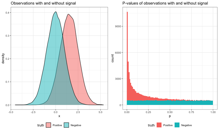
While there is a mixture of positive and negative observations, their values cannot be clearly separated (that would be too easy!) rather noise works against some positives, and some negative observations take on extreme values by chance. This is paralleled by the p-values of positive and negative observations. True positive p-values tend to be small, but may also be large; while true negative p-values are uniformly distributed from 0 to 1 and are as likely to be small as large.
To control the FDR at a level $\alpha$, the Storey procedure first estimates the fraction of null hypothesis (0.5 in our simulation): $\hat{\pi}_{0}$.
This is done by looking at large p-values (near 1). Because large p-values will rarely be signal-containing positives there will be fewer large p-values than would be expected from the number of tests. For example, there are 5106 p-values > 0.9 in our example, which is close to 5000, the value we would expect from $N\pi_{0}*0.1$ (105 * $\pi_{0}$ * 0.1). (I’ll use the true value of $\pi_{0}$ (0.5) as a stand-in for the estimate of $\hat{\pi}_{0}$ so the numbers are a little clearer.)
Just as we expected 5000 null p-values on the interval from [0.9,1], we would expect 5000 null p-values on the interval [0,0.1]. But, there are actually 34415 with p-values < 0.1 because positives tend have small p-values. If we chose 0.1 as a possible cutoff, then we would expect 5000 false positives while the observed number of p-values < 0.1 equals the denominator of the FDR ($\text{FP} + \text{TP}$). The ratio of these two values, 0.145, would be the expected FDR at a p-value cutoff of 0.1. Now, we usually don’t want to choose a cutoff and then live with the FDR we would get, but rather control the FDR at a level $\alpha$ by tuning the cutoff as a parameter $\lambda$.
To apply q-value based FDR control we can use the q-value package:
# install q-value from bioconductor if needed
# remotes::install_bioc("qvalue")

library(qvalue)
qvalue_estimates <- qvalue(simple_pvalue_mixture$p)
The q-value object contains an estimate of $\pi_{0}$ of 0.496 which is close to the true value of 0.5 It also contains a vector of q-values, lFDR, and other goodies.
The q-values are the quantity that we’re usually interested in; if we take all of the q-values less than a target cutoff of say 0.05, then that should give us a set of “discoveries” realizing a 5% FDR.
simple_qvalues <- simple_pvalue_mixture %>%
  mutate(q = qvalue_estimates$qvalues)

fdr_pvalue_cutoff <- max(simple_qvalues$p[simple_qvalues$q < 0.05])

simple_qvalues <- simple_qvalues %>%
  mutate(hypothesis_type = case_when(p <= fdr_pvalue_cutoff & truth == "Positive" ~ "TP",
                                     p <= fdr_pvalue_cutoff & truth == "Negative" ~ "FP",
                                     p > fdr_pvalue_cutoff & truth == "Positive" ~ "FN",
                                     p > fdr_pvalue_cutoff & truth == "Negative" ~ "TN"))

hypothesis_type_counts <- simple_qvalues %>%
  count(hypothesis_type)

TP <- hypothesis_type_counts$n[hypothesis_type_counts$hypothesis_type == "TP"]
FP <- hypothesis_type_counts$n[hypothesis_type_counts$hypothesis_type == "FP"]
FDR <- FP / (TP + FP)

knitr::kable(hypothesis_type_counts) %>%
kableExtra::kable_styling(full_width = FALSE)| hypothesis_type | n |
|---|---|
| FN | 38910 |
| FP | 616 |
| TN | 49384 |
| TP | 11090 |
In this case, due to our simulation, we know whether individual discoveries are true or false positives. As a result we can determine that the realized FDR is 0.053, close to our target of 0.05.
In most cases we would take our discoveries and work with them further, confident that as a population, only ~5% of them are bogus. But, in some cases we care about how likely an individual observation is to be a false positive. In this case we can look at the local density of p-values near an observation of interest to estimate a local version of the FDR, the local FDR (lFDR).
We took advantage of this property during my collaboration with Google Brain aimed to improve the accuracy of peptide matches to proteomics’ spectra using labels from traditional informatics (arXiv). In this study we weighted peptides’ labels with their lFDR using a cross-entropy loss to more strongly penalize failed prediction with high-confidence labels.
lFDR-based shrinkage
Because the lFDR reflects the relative odds that an observation is null it is a useful measure for shrinkage or thresholding aiming to remove noise and better approximate true value. To do this we can weight an observation by 1-lFDR. One interpretation of this is that we are using the lFDR to hedge our bets between the positive and negative mixture components, weighting by our null hypothesis that $\mu$ = 0 with confidence lFDR, and by the alternative $\mu \neq 0$ value of x with confidence 1-lFDR:
\[x_{\text{shrinkage}} = \text{lFDR}\cdot0 + (1-\text{lFDR})\cdot x\]true_values <- tribble(~ truth, ~ mu,
"Positive", beta,
"Negative", 0)
shrinkage_estimates <- simple_qvalues %>%
mutate(lfdr = qvalue_estimates$lfdr,
xs = x*(1-lfdr)) %>%
select(truth, x, xs) %>%
gather(processing, value, -truth) %>%
mutate(processing = case_when(processing == "x" ~ "original value",
processing == "xs" ~ "shrinkage estimate"))
ggplot(shrinkage_estimates, aes(x = value, fill = processing)) +
geom_density(alpha = 0.5) +
geom_vline(data = true_values, aes(xintercept = mu), color = "chartreuse", size = 1) +
facet_grid(truth ~ ., scale = "free_y") +
scale_fill_brewer(palette = "Set1") +
ggtitle("lFDR-based shrinkage improves agreement between observations and the true mean")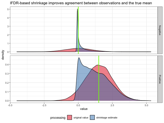
Using lFDR-based shrinkage, values which are just noise were aggressively shrunk toward their true mean of 0 such that there is very little remaining variation. Positives were shrunk using the same methodology retaining extreme values near their measured value. We can verify that there is an overall decrease in uncertainty about the true mean reflecting the removal of noise.
shrinkage_estimates %>%
  inner_join(true_values, by = "truth") %>%
  mutate(resid = value - mu) %>%
  group_by(processing) %>%
  summarize(RMSE = sqrt(mean(resid^2))) %>%
  knitr::kable() %>%
kableExtra::kable_styling(full_width = FALSE)| processing | RMSE |
|---|---|
| original value | 0.9994577 |
| shrinkage estimate | 0.8103141 |
Future Work
In a future post I’ll describe how lFDR-based shrinkage is particularly useful for signal processing of time-resolved peturbation data. In this case, early direct changes are rare, while late indirect changes are quite common. This intuition can be folded into how we estimate the lFDR by estimating a $\hat{\pi}_{0}$ which decreases monotonically with time using the functional FDR.
- Share this on →


