Napistu meets PyTorch Geometric - Predicting Regulatory Interactions with Graph Neural Networks

Biological applications of graph neural networks (GNNs) typically work with either small curated networks (100s-1,000s of nodes) or aggressively filtered subsets of large databases like STRING. The Octopus graph — which I introduced in my previous post — occupies a different space entirely. By integrating eight complementary pathway databases, it creates a genome-scale network with ~50K proteins, metabolites, and complexes spanning ~10M edges, all while preserving rich metadata about edge provenance, confidence scores, and mechanistic detail that filtered approaches discard.

This puts the Octopus in uncharted territory: large enough to capture genome-scale complexity, yet structured enough to preserve the biological interpretability that makes network analysis valuable. GNNs scale well beyond genome-scale requirements (100M+ nodes in social networks), but remain unexplored for comprehensive biological networks that integrate regulatory, metabolic, and interaction data. Bridging this gap requires infrastructure that handles both the biological complexity of multi-source networks and the engineering complexity of training GNNs at scale.

In this post, I’ll introduce Napistu-Torch — the infrastructure that finally makes this space navigable. Available from PyPI and indexed by the Napistu MCP server, Napistu-Torch provides a modular, reproducible framework for training GNNs on comprehensive biological networks. I’ll demonstrate that it’s feasible to train graph convolutional networks on the complete Octopus network using just a laptop (albeit with 2 days of training time for the full suite of models). But the real contribution is the ecosystem: the data structures, pipelines, and evaluation strategies that unlock far more sophisticated analyses.

Specifically, I’ll walk through the key components of the Napistu-Torch ecosystem:

• Data engineering: Converting NapistuGraph objects into PyTorch Geometric Data objects while preserving the Octopus network’s rich vertex and edge metadata. The NapistuDataStore manages caching and lazy loading of derived artifacts, eliminating the overhead of rebuilding datasets — you can immediately start training or evaluating models.

• Model components: Breaking down the anatomy of a GNN into its core building blocks — encoders that learn vertex representations via message passing, heads that make predictions from embeddings, and optional edge encoders that weight edges based on metadata. I’ll compare several architectures (GCN, GraphSAGE, GraphConv) with and without edge encoding.

• Training infrastructure: Leveraging PyTorch Lightning to orchestrate model training with minimal boilerplate. Configuration files define entire experiments, making it easy to reproduce results or modify architectures without touching code. The CLI supports the full train-test workflow with automatic experiment tracking via Weights & Biases.

• Self-supervised learning: Training without ground truth labels by framing the task as edge prediction. The key challenge is forcing the model to learn real biological patterns through careful negative sampling — ensuring that negative examples aren’t trivially distinguishable from true edges while remaining computationally tractable at the scale of millions of edges.

• Model interpretation: Evaluating what the models learn through three lenses: (1) vertex embeddings that capture molecular similarity and pathway membership, (2) learned edge weights that reveal what makes a high-confidence interaction, and (3) edge prediction patterns that assess whether the model is learning biological structure versus discovering topological constraints.

From Napistu to PyTorch Geometric

Graph neural networks learn representations of nodes and edges by iteratively aggregating information from local neighborhoods — a process called message passing. Unlike traditional neural networks that operate on fixed-size inputs, GNNs can handle graphs of arbitrary size and structure, making them well-suited for biological networks where connectivity patterns encode meaningful relationships. Through multiple rounds of message passing, GNNs capture increasingly complex structural patterns, from immediate neighbors to broader network motifs.

Graph neural networks in Python typically use PyTorch Geometric (PyG), a library that extends PyTorch with data structures and operations optimized for graph-structured data. PyG represents graphs using the Data class, which stores node features, edge connectivity, and optional edge attributes as PyTorch tensors — the fundamental format needed for GPU-accelerated training.

Napistu networks, however, live in a different ecosystem. A NapistuGraph (subclass of igraph.Graph) stores biological networks with rich vertex and edge metadata—species types, reaction mechanisms, database provenance, confidence scores. Training GNNs on these networks requires bridging these two worlds: preserving Napistu’s biological metadata while converting graphs into PyG’s tensor-based format.

This is where Napistu-Torch comes in. Following the same design philosophy as Napistu-Py — extending established frameworks rather than reinventing them — Napistu-Torch builds on PyG with biology-aware data structures and methods. The goal is to lean on well-established frameworks like PyG, PyTorch Lightning, and Weights & Biases so the codebase can focus on domain-specific challenges: encoding biological signals, integrating diverse metadata, and evaluating models with biologically meaningful metrics

NapistuGraph → NapistuData

A key data structure in Napistu-Torch is NapistuData, which extends PyG’s Data class to handle biological network metadata. At its core, it contains the same PyTorch tensor components that any PyG model expects:

• x: vertex attributes [# vertices × # of vertex features]
• edge_index: graph connectivity [2 × # of edges]
• edge_attr (optional): edge attributes [# edges × # of edge features]
• edge_weight (optional): edge weights [# of edges × 1]
• y (optional): node labels for supervised tasks [# of vertices × 1]

But NapistuData also tracks Napistu-specific metadata—feature encoders, vertex and edge masks for train/val/test splits, and mappings back to the original NapistuGraph identifiers.

Creating a NapistuData

Constructing a NapistuData instance involves three conceptual steps:

1. Load the network: Start with a NapistuGraph and its associated SBML_dfs database — here, the 8-source Octopus consensus network downloaded from Google Cloud Storage
2. Augment with attributes: Add relevant vertex and edge metadata as described in the Octopus network post
3. Encode as tensors: Convert attributes to torch.Tensors using sklearn-based encoders with automatic type detection (binary→passthrough, categorical→one-hot, continuous→standardization) and train/val/test splitting

In practice, you rarely construct NapistuData objects manually. Instead, the NapistuDataStore handles this process automatically — loading raw data, applying transformations, caching results, and managing related artifacts. This is what enables immediate model training without rebuild overhead. I’ll demonstrate the store-based workflow after covering environment setup.

Following along

This analysis is fully reproducible — all code, data, and model configurations are provided so you can run the complete workflow on your own machine. This section covers environment setup and file locations.

Environment setup

To reproduce this notebook:

1. Install uv (or use pip if preferred).

2. Set up a Python environment:

uv venv --python 3.11
source .venv/bin/activate
# Core dependencies
uv pip install torch==2.8.0
uv pip install torch-scatter torch-sparse -f https://data.pyg.org/whl/torch-2.8.0+cpu.html
uv pip install napistu==0.7.5
uv pip install "napistu-torch[pyg,lightning]==0.2.6"
# if you'd like to render the notebook, you'll need to install these additional dependencies
uv pip install seaborn ipykernel nbformat nbclient umap-learn
python -m ipykernel install --user --name=blog-staging

1. Download the napistu_nets.qmd notebook (or copy and paste the relevant code blocks).

2. Choose your path:

   • 4a. Using pre-trained models (recommended): Download pre-trained models and configs (~50MB) and extract to your experiments directory.
   • 4b. Training from scratch: Download model configs only to train models yourself (requires ~2 days on an M4 Max MacBook Pro, 8-12 hours per model).

3. Configure EXPERIMENTS_DIR and other paths in the env_setup code block to point to your local directories.

Configuration and imports

# imports

import logging
import os
import re
from pathlib import Path

import numpy as np
from matplotlib.colors import LogNorm
import matplotlib.pyplot as plt
import pandas as pd
import torch
import seaborn as sns

from napistu_torch.evaluation.edge_prediction import summarize_edge_predictions_by_strata, plot_edge_predictions_by_strata
from napistu_torch.evaluation.edge_weights import compute_edge_feature_sensitivity, format_edge_feature_sensitivity, plot_edge_feature_sensitivity
from napistu_torch.evaluation.evaluation_manager import EvaluationManager
from napistu_torch.evaluation.model_comparison import compare_embeddings
from napistu_torch.evaluation.pathways import calculate_pathway_similarities
from napistu_torch.lightning.tasks import get_edge_encoder
from napistu_torch.lightning.workflows import predict
from napistu_torch.load.gcs import gcs_model_to_store
from napistu_torch.utils.torch_utils import select_device
from napistu_torch.visualization.basic_metrics import plot_model_comparison
from napistu_torch.visualization.embeddings import layout_umap, plot_coordinates_with_masks

logging.basicConfig(level=logging.INFO)
logger = logging.getLogger("napistu_torch")

# globals

OVERWRITE = False

EXPERIMENTS_DIR = Path(os.path.expanduser("~/Desktop/EXPERIMENTS/20251106_edge_prediction"))
NAPISTU_DATA_DIR = os.path.join(EXPERIMENTS_DIR, ".napistu_data")
STORE_DIR = os.path.join(EXPERIMENTS_DIR, ".store")
CACHE_DIR = EXPERIMENTS_DIR

EXPERIMENTS = [
    # leave this as a list so it defines plot order
    "20251106_gcn_baseline",
    "20251106_gcn_edge_encoding",
    "20251106_sage_baseline",
    "20251106_graphconv_baseline",
    "20251106_graphconv_edge_encoding"
]

EXPERIMENT_LABELS = {
    "20251106_gcn_baseline" : "GCN",
    "20251106_gcn_edge_encoding" : "GCN + Edge Encoding",
    "20251106_sage_baseline" : "SAGE",
    "20251106_graphconv_baseline" : "GraphConv",
    "20251106_graphconv_edge_encoding" : "GraphConv + Edge Encoding"
}

ordered_labels = [EXPERIMENT_LABELS[exp] for exp in EXPERIMENTS]

TOP_MODEL_NAME = "GraphConv + Edge Encoding"
EMBEDDING_COMPARISONS_PATH = CACHE_DIR / "embedding_comparisons.tsv"

# validation
if not os.path.isdir(EXPERIMENTS_DIR):
    raise FileNotFoundError(f"Experiments directory not found: {EXPERIMENTS_DIR}")
if not os.path.isdir(CACHE_DIR):
    raise FileNotFoundError(f"Cache directory not found: {CACHE_DIR}")

Managing artifacts with NapistuDataStore

Training and evaluating GNN models requires more than just the graph structure — we need encoded features, train/val/test splits, pathway metadata for evaluation, and edge stratification data for negative sampling. Building these artifacts from scratch involves loading the full SBML_dfs database (several minutes) and running various preprocessing steps. Doing this repeatedly during development would be painfully slow.

The NapistuDataStore solves this by managing a registry of cached artifacts. Once built, artifacts load in seconds rather than minutes. Named artifact definitions in the napistu_torch.load.artifacts module support common workflows and integrate seamlessly with config-driven training.

Importantly, the store provides a clean abstraction layer over Napistu-Py. All the logic for loading SBML databases, decorating graphs with metadata, and extracting biological annotations is baked into Napistu-Torch objects. Users can work entirely with NapistuData, encoders, and dataloaders without ever touching Napistu-Py code — though if you’re curious about the underlying biological data model, Napistu-Py is pretty cool.

Initializing the store

A store can be initialized directly from one of the bundled Napistu networks on Google Cloud Storage using gcs_model_to_store. This creates and manages two local directories:

• napistu_data_dir: Raw data including the NapistuGraph and SBML_dfs
• store_dir: Cached artifacts and the registry file tracking what’s been built

napistu_data_store = gcs_model_to_store(
    napistu_data_dir = NAPISTU_DATA_DIR,
    store_dir = STORE_DIR,
    asset_name = "human_consensus",
    # pin to a stable version of the dataset for reproducibility
    asset_version = "20250923" 
)

Building and caching artifacts

The ensure_artifacts method checks whether requested artifacts exist and builds any that are missing. For this analysis, we need four artifacts:

napistu_data_store.ensure_artifacts([
    "edge_prediction",
    "comprehensive_pathway_memberships",
    "edge_strata_by_node_type",
    "edge_strata_by_node_species_type"
])

These artifacts are:

• edge_prediction: A NapistuData instance with train/val/test edge masks, used for self-supervised learning
• comprehensive_pathway_memberships: Detailed pathway associations for all vertices (including fine-grained Reactome pathways), used for evaluating whether embeddings capture biological organization
• edge_strata_by_node_type: Edge categories based on source/target node types (species→species, species→reaction, etc.), used for stratified negative sampling
• edge_strata_by_node_species_type: Finer-grained edge categories including species types (protein, metabolite, RNA), used for assessing prediction biases

Once built, these artifacts load almost instantly:

napistu_data = napistu_data_store.load_napistu_data("edge_prediction")
comprehensive_pathway_memberships = napistu_data_store.load_vertex_tensor("comprehensive_pathway_memberships")
edge_strata_by_node_type = napistu_data_store.load_pandas_df("edge_strata_by_node_type")
edge_strata_by_node_species_type = napistu_data_store.load_pandas_df("edge_strata_by_node_species_type")

    INFO:napistu_torch.napistu_data_store:Loading NapistuData from /Users/sean/Desktop/EXPERIMENTS/20251106_edge_prediction/.store/napistu_data/edge_prediction.pt
    INFO:napistu_torch.napistu_data_store:Loading VertexTensor from /Users/sean/Desktop/EXPERIMENTS/20251106_edge_prediction/.store/vertex_tensors/comprehensive_pathway_memberships.pt
    INFO:napistu_torch.napistu_data_store:Loading pandas DataFrame from /Users/sean/Desktop/EXPERIMENTS/20251106_edge_prediction/.store/pandas_dfs/edge_strata_by_node_type.parquet
    INFO:napistu_torch.napistu_data_store:Loading pandas DataFrame from /Users/sean/Desktop/EXPERIMENTS/20251106_edge_prediction/.store/pandas_dfs/edge_strata_by_node_species_type.parquet

The store abstraction means that downstream code (training scripts, evaluation notebooks) can simply request artifacts by name without worrying about paths, versions, or rebuild logic.

Anatomy of a GNN

Training a GNN requires coordinating several components: the model architecture itself, the task definition, data management, and training infrastructure. This section breaks down each component — starting with a conceptual overview of what it does, then showing how it’s implemented in Napistu-Torch. We’ll begin with the high-level system architecture, then work through the task definition, model components (encoder, head, edge encoder), and finally the training infrastructure that orchestrates everything.

System architecture

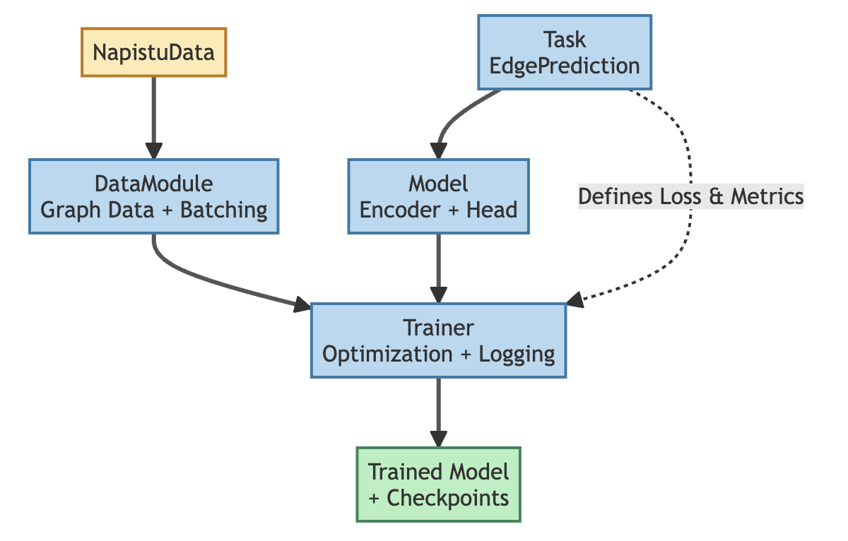
Training deep learning models involves coordinating several standard components: the Task defines what we’re learning (loss function, metrics), the Model implements the neural network architecture, the DataModule handles data loading and batching, and the Trainer orchestrates the optimization loop. Each component is configured independently, providing modularity and clear separation of concerns.

The following subsections examine how these components work in the context of biological network analysis, covering the task definition (edge prediction), model architecture (GNN encoders and heads), and training infrastructure. Later, in the Workflow Management section, I’ll show how Napistu-Torch packages these component-level configs into a single ExperimentConfig for experiment reproducibility.

Task: what are we trying to predict?

At the highest level, a GNN task defines the learning objective — what predictions we want the model to make and how we’ll evaluate its performance. Different tasks require different architectural components and training strategies. Common GNN tasks include node classification (predicting properties of individual nodes), graph classification (predicting properties of entire graphs), and edge prediction (predicting whether edges should exist between nodes).

Edge prediction in Napistu-Torch. For this analysis, we’re using the edge prediction task (also called link prediction). The goal is to predict whether an edge should exist between two nodes in a biological network. This is particularly valuable for discovering potential protein-protein interactions, metabolic relationships, or regulatory connections that may be missing from current databases. Crucially, edge prediction is self-supervised — it doesn’t require vertex or edge labels, which are often difficult to obtain or overly contrived for biological networks.

The training process works by teaching the model to discriminate between:

• Positive edges: Real edges that exist in the training set
• Negative edges: Node pairs sampled as non-edges (chosen to maintain biological plausibility)

The EdgePredictionTask class in Napistu-Torch orchestrates this process, handling negative sampling, computing the loss function (binary cross-entropy), and evaluating performance using metrics like AUC and average precision. The task operates in a transductive setting — the model generates node embeddings using only training edges for message passing; validation and test edges are excluded from neighborhood aggregation but used as supervision to evaluate the decoder’s edge predictions.

Naïve negative sampling (randomly pairing vertices) produces trivially distinguishable negatives. Early models without stratification quickly reached >0.95 AUC by exploiting two artifacts: (1) sampling impossible edge types like reaction→reaction that never occur in real edges, and (2) sampling random pairs that ignore the highly variable degree distribution of biological networks, making hub nodes easy to memorize.

The NegativeSampler addresses this by tracking edge attributes — such as combinations of from- and to-node types and degree distributions within each stratum. It generates negative samples that match both the observed edge strata and vertex in- and out-degree distributions, forcing the model to learn biological patterns rather than graph artifacts.

For the models trained here, I use coarse-grained node-type strata (species vs. reaction), sampling negatives to match the observed proportions of species→species, species→reaction, and reaction→species. Finer-grained stratification — matching entity types like protein vs. complex vs. metabolite — could further reduce imbalances, but at a cost: more strata mean sampling separately from dozens of pools during batch construction, limiting vectorization efficiency.

With the task defined, let’s examine the three core model components: the encoder that learns node embeddings, the head that produces predictions, and the optional edge encoder that can weight message passing.

Encoder: learning vertex representations

The encoder is the core of a GNN — it transforms raw node features into learned embeddings by aggregating information from each node’s local neighborhood. Through multiple layers of message passing, encoders capture increasingly complex patterns of connectivity and feature similarity. The encoder’s architecture determines how information flows through the graph and what kinds of structural patterns the model can learn.

Message passing encoders in Napistu-Torch. Napistu-Torch leverages PyG’s library of encoder architectures, wrapping them through the MessagePassingEncoder class for easy configuration:

• GraphSAGE (SAGE)
  • Samples and aggregates features from neighbors using various aggregation functions (mean, max, add)
  • Efficient and scalable, well-suited for large biological networks
  • Does not support edge weighting — treats all edges uniformly
• GraphConv
  • Similar to SAGE with a simplified message passing scheme
  • Supports optional edge weighting
• Graph Convolutional Networks (GCN)
  • Uses symmetric normalization that accounts for node degrees
  • Supports edge weighting

All encoders follow a multi-layer architecture, progressively refining node embeddings through repeated neighborhood aggregation. The framework provides a unified interface, allowing you to swap architectures through configuration files without changing code.

Head: making predictions from embeddings

Once the encoder has produced node embeddings, the head (or decoder) transforms these embeddings into task-specific predictions. The head’s role is to adapt the general-purpose embeddings produced by the encoder to the specific prediction task — edge prediction, node classification, graph classification, etc.

Heads in Napistu-Torch. For edge prediction, the most commonly used head is the dot product, which computes the inner product of source and target node embeddings — assuming that nodes with similar embeddings should be connected. This is the simplest and most efficient option, serving as a strong baseline in most GNN edge prediction work. Napistu-Torch also implements more expressive alternatives (MLP, bilinear) that can learn non-linear relationships between node pairs, though these come with increased computational cost.

For this analysis, all models use the dot product head due to its efficiency on large biological networks and strong empirical performance. Napistu-Torch also provides heads for other tasks like node classification, all accessible through configuration files.

The dot product head is symmetric — it treats vertex A→B identically to B→A — making it well-suited for undirected interactions but poorly suited for regulation, where the roles of regulator and target fundamentally differ. Asymmetric heads like DistMult could address this by learning distinct representations for source and target vertices, enabling the model to differentiate regulators from their targets.

However, even asymmetric heads may struggle to take advantage of Napistu’s diverse edge types: protein-protein interactions, activation, inhibition, catalysis, and more. An asymmetric model could implicitly learn these cues, but the meaning of a high prediction score would remain ambiguous: is it activation, inhibition, binding?

Relation-aware heads like RotatE offer a more promising path. Originally developed for knowledge graph completion, these architectures explicitly model edge types as distinct relations, learning separate transformation rules for each. This approach enables the model to capture the principles of regulation directly, discerning activators from inhibitors and regulators from binding partners. Rather than merely predicting edges, these models yield typed edges — specific, testable hypotheses about the nature of regulatory relationships.

Edge encoder: weighting message passing

While many GNN implementations either ignore edge attributes entirely or only accept a single edge weight, biological networks often have rich edge metadata. The challenge is that most message passing architectures (like SAGE) don’t support edge attributes at all, while others (like GCN and GraphConv) only accept a single scalar weight per edge.

Learned edge weighting in Napistu-Torch. Napistu-Torch addresses this through the EdgeEncoder class, which compresses multi-dimensional edge attributes into a single learned weight that modulates message passing strength. The edge encoder is a lightweight MLP that takes edge features as input and outputs a scalar weight in [0, 1] via sigmoid activation. These learned weights control how strongly each edge contributes during neighborhood aggregation.

This approach filters noisy edges and amplifies reliable ones, focusing message passing on the most informative connections — crucial in biological networks where edge quality varies widely. The encoder trains end-to-end with the rest of the model, learning which edge attributes are most predictive for the task while remaining compatible with standard GNN architectures that expect scalar edge weights.

Model overview

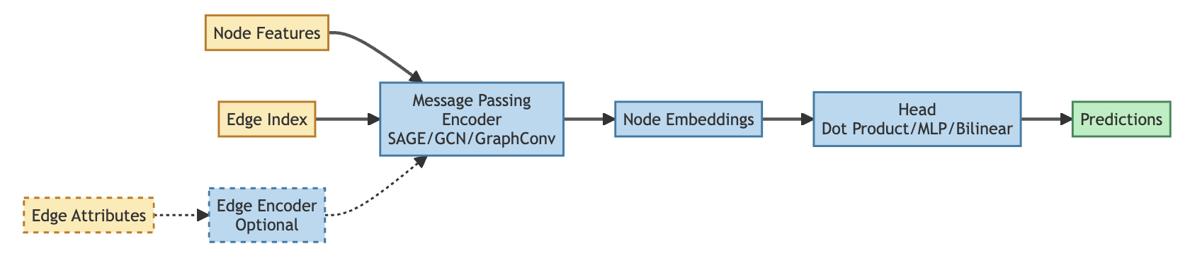
The diagram shows how model components connect during a forward pass. Node features and edge connectivity flow through the message passing encoder to produce node embeddings. The head then transforms these embeddings into task-specific predictions — edge scores for edge prediction, class probabilities for node classification.

The optional edge encoder (shown in dashed lines) learns to weight edges based on edge attributes, modulating how strongly each edge contributes during message passing. This is particularly useful when edge reliability varies across data sources, as in the Octopus network.

These model components (encoder, head, edge encoder) define the core prediction logic, but training a GNN requires additional infrastructure to manage data loading, optimization, and evaluation. Napistu-Torch uses PyTorch Lightning to orchestrate this training workflow.

Training infrastructure: PyTorch Lightning

While the core GNN components (encoder, head, task) are pure PyTorch, actually training a model requires substantial boilerplate: optimizer setup, learning rate scheduling, checkpoint saving, logging metrics, handling different hardware accelerators, and coordinating training/validation loops.

Lightning integration in Napistu-Torch. Napistu-Torch uses PyTorch Lightning to handle this training infrastructure automatically. Lightning separates scientific code (model architecture, loss functions) from engineering code (training loops, GPU management), making experiments more reproducible and less error-prone.

The key Lightning components are:

• LightningModule: Wraps the core task (encoder + head) and defines training/validation steps, metrics computation, and optimizer configuration. Napistu-Torch provides task-specific adapters like EdgePredictionLightning that bridge pure PyTorch implementations with Lightning’s training infrastructure.

• Trainer: Orchestrates the training loop, handles checkpointing, manages device placement (CPU/GPU/MPS), integrates with experiment tracking tools like Weights & Biases, and implements callbacks like early stopping.

With this architecture, you can concentrate on defining model and task logic, while Lightning takes care of all training mechanics.

Data management: batching strategies

The NapistuDataModule is Lightning’s interface for data loading. It can be initialized directly from an ExperimentConfig, automatically handling artifact loading from the NapistuDataStore, data validation, and dataloader creation.

Full-batch vs. mini-batch training. Napistu-Torch provides two DataModule implementations with fundamentally different training strategies:

• FullGraphDataModule: Returns the complete graph in each batch, processing all training edges simultaneously for a single gradient update per epoch. With only one update per epoch, the model can converge prematurely before exploring the optimization landscape effectively.

• EdgeBatchDataModule: Splits training edges into mini-batches while still using all training edges for message passing. Each batch computes loss and gradients on a subset of training edges but uses the full graph structure for neighborhood aggregation. This enables multiple gradient updates per epoch by subdividing the supervision signal — effectively trading fewer epochs for more updates per epoch, allowing more thorough optimization.

For the models in this post, I used EdgeBatchDataModule with 20 batches per epoch, meaning the model updates its weights 20 times per epoch rather than once.

Workflow management

For this post, I’m comparing 5 models across different encoder architectures and edge encoding strategies:

• GraphConv (+/- edge encoding)
• GCN (+/- edge encoding)
• SAGE (edge encoding not supported)

These models use identical hyperparameters (200 epochs, same batch configuration, same hidden dimensions) for a fair comparison. These models are deliberately unoptimized, with no hyperparameter tuning and simple dot-product heads, as the focus is on feasibility and infrastructure rather than peak performance.

Training configuration in Napistu-Torch. The ExperimentConfig composes lower-level Pydantic configs (DataConfig, ModelConfig, TaskConfig, TrainerConfig, WandBConfig) with validation and sensible defaults. Define an experiment in a minimal YAML file, inherit defaults automatically.

The Napistu-Torch CLI supports training and testing directly from the command line:

napistu-torch train graphconv_baseline.yaml --out-dir 20251106_graphconv_baseline
napistu-torch test 20251106_graphconv_baseline

Training/validation/test metrics log to Weights & Biases for easy comparison across experiments. Each run saves a RunManifest containing the Weights & Biases run ID and complete ExperimentConfig (with all defaults expanded), making experiments fully reproducible.

The configs and training script for these 5 models are available here. On an M4 Max MacBook Pro with 48GB of RAM, training the full suite takes ~2 days (~8-12 hours per model).

PyTorch’s Metal Performance Shaders (MPS) backend enables GPU acceleration on Apple Silicon, though support is less mature than CUDA. For these experiments, MPS performed well on simpler models, but when training models with edge encoders near my machine’s memory limits, I encountered sporadic tensor corruption. I trained those models on CPU instead—a reasonable fallback since the irregular memory access patterns of message passing (variable numbers of messages per node) meant the performance gap between CPU and GPU was modest for these network sizes.

Now let’s load these trained models and compare their performance.

Model comparison

Model evaluation in Napistu-Torch. The EvaluationManager class loads a run’s RunManifest and provides methods for accessing checkpoints, the NapistuDataStore, and Weights & Biases metrics — eliminating the need for manual path management or API queries. Here, I’ll load all five trained models and compare their performance metrics and learned representations.

eval_managers = {
    EXPERIMENT_LABELS[out_dir]: EvaluationManager(EXPERIMENTS_DIR / out_dir) for out_dir in EXPERIMENTS
}

# Extract model summaries directly from Weights & Biases using their API
run_summaries = {exp: manager.get_run_summary() for exp, manager in eval_managers.items()}

# visualize model comparison
fig, (ax1, ax2) = plot_model_comparison(run_summaries, ordered_labels)

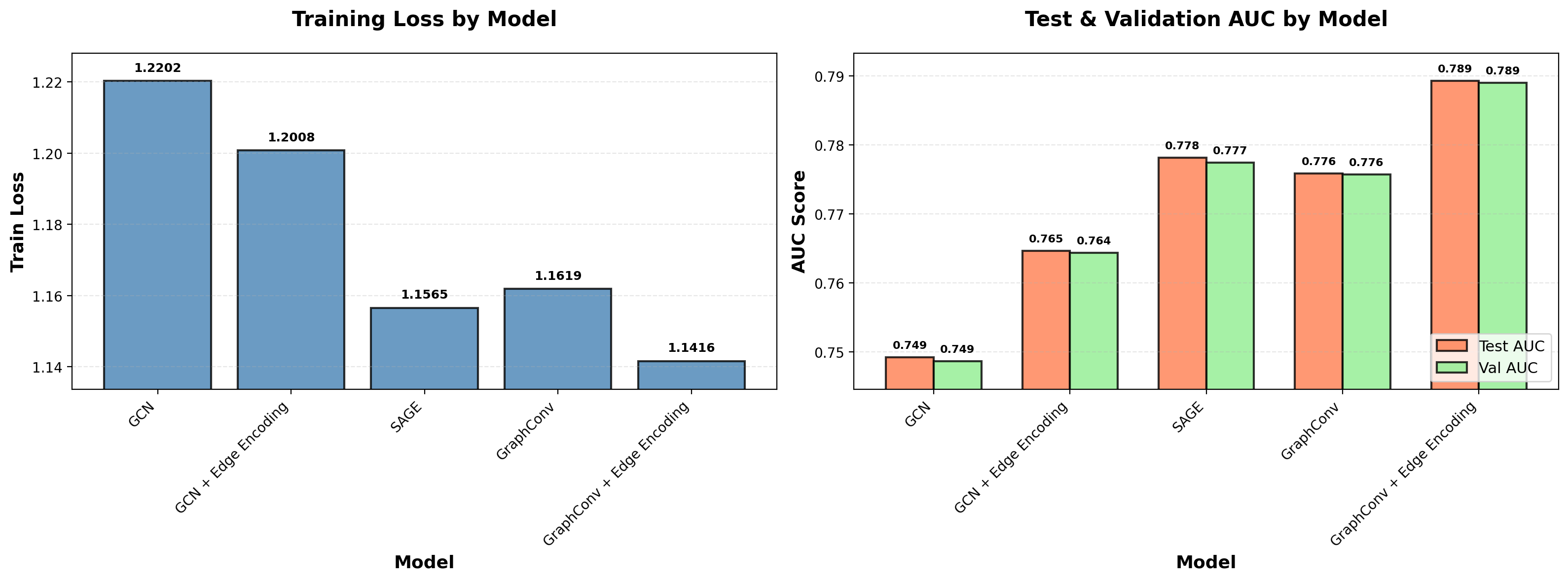
The training loss shown is the final epoch’s binary cross-entropy, aggregated across all mini-batches, computed on equal numbers of real edges (70% of the network) and negative samples. Validation AUC measures how well the model ranks held-out real edges (15% of the network, excluded from message passing) above an equal number of negative samples. This metric is evaluated after each epoch for checkpoint selection and early stopping. Test AUC evaluates the same ranking task on the final 15% of edges.

Performance differences across models are modest but consistent. Encoder architecture matters: SAGE > GraphConv >> GCN. Edge encoding provides a clear improvement across architectures that support it. While these models haven’t been optimized — no hyperparameter tuning, simple dot product heads—the consistent trends across architectures validate the training infrastructure and provide a baseline for future work.

Next, I’ll compare the learned representations across models. Specifically: Do different encoder architectures produce similar vertex embeddings? Do models with edge encoders learn comparable edge weights? These comparisons reveal whether the biological signal is robust to architectural choices or whether different models capture fundamentally different patterns.

top_model_manager = eval_managers[TOP_MODEL_NAME]
napistu_data = top_model_manager.load_napistu_data()
napistu_data_store = top_model_manager.get_store()
napistu_graph = napistu_data_store.load_napistu_graph()

# pull out the node types and create a mask to distinguish species and reactions
node_types = napistu_graph.get_vertex_series("node_type")
is_species_mask = (node_types == "species").values

## Extract model embeddings
edge_encodings = {}
species_embeddings = {}
for exp, evaluation_manager in eval_managers.items():
    # load the model and data
    model = evaluation_manager.load_model_from_checkpoint()
    napistu_data = evaluation_manager.load_napistu_data()
    
    # pull out learned edge weights (if an edge encoder is present)
    if model.task.encoder.edge_weighting_type == "learned_encoder":
        edge_encodings[exp] = model.get_learned_edge_weights(napistu_data)
    
    # pull out the vertex embeddings
    embeddings = model.get_embeddings(napistu_data)
    species_embeddings[exp] = embeddings[is_species_mask]

    # cleanup
    evaluation_manager.experiment_dict = None

Comparing vertex embeddings

To compare vertex embeddings across models, I compute species-species cosine similarities within each model’s embedding space (# species × hidden dimension), then calculate the Spearman correlation between these similarity matrices across model pairs. This approach works regardless of embedding dimension and avoids the need for explicit alignment (e.g., Procrustes rotation).

def create_correlation_heatmap(
    embedding_comparisons: pd.DataFrame,
    model_order: list[str] | None = None
) -> pd.DataFrame:
    
    # Get all unique models
    all_models = (
        set(embedding_comparisons['model1'].unique()) | \
        set(embedding_comparisons['model2'].unique())
    )
    
    # Use provided order or default to sorted
    if model_order is None:
        models = sorted(all_models)
    else:
        # Validate that all models in data are in the provided order
        missing_models = all_models - set(model_order)
        if missing_models:
            raise ValueError(f"Models in data but not in model_order: {missing_models}")
        # Use only models that exist in the data, in the specified order
        models = [m for m in model_order if m in all_models]
    
    # Initialize matrix with 1s on diagonal
    corr_matrix = pd.DataFrame(
        np.eye(len(models)),
        index=models, 
        columns=models
    )
    
    # Fill in the correlations (both upper and lower triangles)
    for _, row in embedding_comparisons.iterrows():
        corr_matrix.loc[row['model1'], row['model2']] = row['spearman_rho']
        corr_matrix.loc[row['model2'], row['model1']] = row['spearman_rho']
    
    return corr_matrix

# compute the embedding comparisons (cached since this takes a few minutes to run)

if os.path.isfile(EMBEDDING_COMPARISONS_PATH) and not OVERWRITE:
    embedding_comparisons = pd.read_csv(EMBEDDING_COMPARISONS_PATH, sep="\t", index_col=0)
else:
    device = select_device(mps_valid = True)
    embedding_comparisons = compare_embeddings(species_embeddings, device)
    embedding_comparisons.to_csv(EMBEDDING_COMPARISONS_PATH, sep="\t", index_col=False)

# visualize the embedding comparisons

corr_matrix = create_correlation_heatmap(embedding_comparisons, model_order=ordered_labels)

# Display as heatmap
mask = np.triu(np.ones_like(corr_matrix, dtype=bool), k=1)

plt.figure(figsize=(10, 8))
sns.heatmap(
    corr_matrix,
    annot=True,
    fmt='.3f',
    cmap='RdYlBu_r',
    mask=mask,
    vmin=0,
    vmax=1,
    square=True,
    cbar_kws={'label': 'Spearman ρ'},
)
plt.title(
    'Vertex embedding similarity across models',
    fontsize=15,
    fontweight='bold',
    pad=20,
    loc='left'
)
plt.tight_layout()
plt.show()

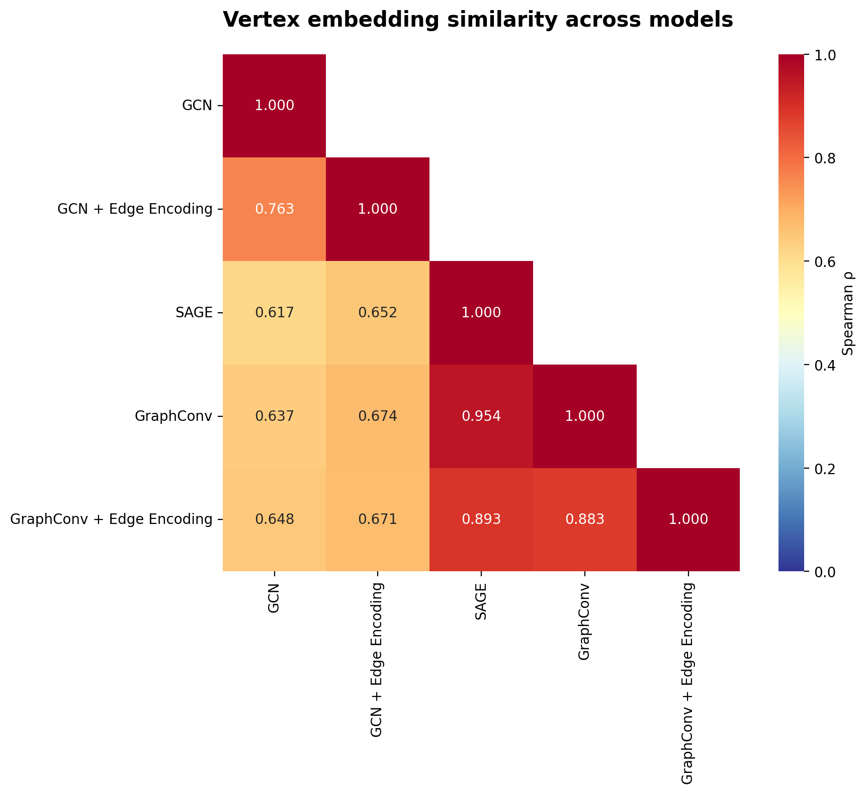
All models produce highly correlated embeddings (ρ > 0.6 across all pairs), indicating they’ve captured similar biological structure despite architectural differences. However, encoder choice does matter: GCN embeddings correlate less strongly with GraphConv/SAGE (ρ ≈ 0.6-0.7) than GraphConv and SAGE correlate with each other (ρ ≈ 0.9). This suggests that while all models learn similar biological signals, GCN’s symmetric normalization produces somewhat different vertex representations than the mean aggregation used by GraphConv and SAGE.

Comparing learned edge weights

As I’ve previously discussed, confidence in regulatory interactions varies greatly across data sources, and edge weights should capture this uncertainty for downstream network analysis. However, determining appropriate edge weights is challenging when multiple data source attributes each capture different aspects of reliability.

The edge encoder provides a way to learn what makes a high-confidence edge empirically. While I’ll examine the learned edge features in detail later, here I’ll assess whether edge weights are consistent across model architectures by directly comparing the ~10M learned weights from GCN + edge encoding and GraphConv + edge encoding.

Since visualizing 10M points requires aggregation, I’ll use a hexbin plot (bivariate histogram) with logit-transformed weights to map the sigmoid outputs back to ℝ:

def safe_logit(p: torch.Tensor, eps: float = 1e-7) -> torch.Tensor:
    p = torch.clamp(p, eps, 1 - eps)
    return torch.log(p / (1 - p))

def plot_edge_encoding_hexbin(
    tensor1: torch.Tensor,
    tensor2: torch.Tensor,
    label1: str = "Model 1",
    label2: str = "Model 2",
    transform_to_logit: bool = True,
    gridsize: int = 50,
    cmap: str = 'viridis',
    figsize: tuple = (10, 8),
) -> tuple:
    # Apply logit transformation if requested
    if transform_to_logit:
        tensor1 = safe_logit(tensor1)
        tensor2 = safe_logit(tensor2)
    
    # Convert to numpy
    if torch.is_tensor(tensor1):
        x = tensor1.cpu().numpy()
    else:
        x = np.array(tensor1)
    
    if torch.is_tensor(tensor2):
        y = tensor2.cpu().numpy()
    else:
        y = np.array(tensor2)
    
    # Create figure
    fig, ax = plt.subplots(figsize=figsize)
    
    # Create hexbin plot with log-scaled color
    hexbin = ax.hexbin(
        x, y,
        gridsize=gridsize,
        cmap=cmap,
        mincnt=1,
        norm=LogNorm()
    )
    
    # Add colorbar
    cb = plt.colorbar(hexbin, ax=ax)
    cb.set_label('Count (log scale)', fontsize=12, fontweight='bold')
    
    # Labels and title
    ax.set_xlabel(label1, fontsize=13, fontweight='bold')
    ax.set_ylabel(label2, fontsize=13, fontweight='bold')
    ax.set_title(
        'Learned edge weight similarity across models',
        fontsize=15,
        fontweight='bold',
        pad=20,
        loc='left'
    )
    
    # Add diagonal reference line (y=x)
    min_val = min(x.min(), y.min())
    max_val = max(x.max(), y.max())
    ax.plot(
        [min_val, max_val],
        [min_val, max_val],
        'r--',
        alpha=0.5,
        linewidth=2,
        label='y=x'
    )
    ax.legend(loc='upper left', fontsize=11)
    
    # Equal aspect ratio
    ax.set_aspect('equal', adjustable='box')
    
    plt.tight_layout()
    
    return fig, ax

fig, ax = plot_edge_encoding_hexbin(
    edge_encodings["GCN + Edge Encoding"],
    edge_encodings["GraphConv + Edge Encoding"],
    label1="GCN + Edge Encoding",
    label2="GraphConv + Edge Encoding",
    transform_to_logit=True,
    gridsize=50,
    cmap='viridis'
)
plt.show()

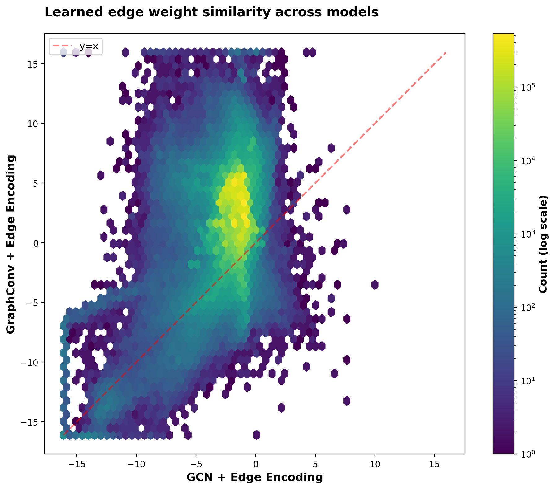
The edge encoder paired with GraphConv uses a wider dynamic range (logit -5 to 7, corresponding to sigmoid weights 0.007-0.999) compared to GCN + edge encoder (logit -3 to 0, corresponding to 0.05-0.5). This means GraphConv’s edge encoder more thoroughly distinguishes between low-, medium-, and high-confidence edges. Both model-encoder combinations agree on which edges to effectively ignore (lower-left quadrant, sigmoid weights < 0.05), but differ in how strongly they upweight reliable edges.

Having established these cross-model comparisons, I’ll now examine the top-performing model (GraphConv + edge encoding) in detail to understand what biological patterns it has captured and where its limitations lie.

Evaluating the top model

Having compared models on performance and learned representations, I’ll now examine what the best-performing model (GraphConv + edge encoding) has actually learned. GNN-based edge prediction offers three potential contributions beyond predicting missing edges:

1. Vertex embeddings capture molecular similarity - Embeddings group similar vertices across entity types, enabling community detection and direct similarity queries. Community detection could identify functional modules — sets of proteins, metabolites, and reactions that cluster together in the embedding space. Similarity queries could assess how closely any two entities resemble each other, even across different entity types.

2. Learned edge weights for network analysis - The edge encoder learns weights that reflect edge reliability, potentially replacing hand-crafted heuristics in downstream analyses like network layouts, shortest paths, propagation algorithms, and shallow embedding methods. For multi-source networks like the Octopus, this is particularly valuable, rather than manually deciding how to weight STRING coexpression scores versus IntAct citation counts, the model learns what combinations of edge attributes indicate reliability.

3. Edge predictions for hypothesis generation - While self-supervised training is the primary motivation for edge prediction, the predictions themselves may identify plausible regulatory connections absent from current databases. This becomes more promising with expressive heads that can model directional regulation rather than the symmetric similarity assumed by the dot product.

I’ll explore each of these potential contributions using the GraphConv + edge encoding model.

Molecular similarity

Embedding structure

To assess the structure of the vertex embeddings, I’ll use UMAP to project the 128-dimensional embeddings into 2D, then overlay vertex attributes to explore what determines similarity in the embedding space.

embeddings = species_embeddings[TOP_MODEL_NAME]
umap_layout_species = layout_umap(embeddings, n_neighbors=20)

mask = [bool(re.search("__species_type", x)) for x in napistu_data.get_vertex_feature_names()]
indices = [i for i, m in enumerate(mask) if m]
masks = napistu_data.x[:, indices]

# only look at the vertices with embedding values
masks = masks[is_species_mask]
mask_names = [x for x, m in zip(napistu_data.get_vertex_feature_names(), mask) if m]

# drop empty masks
empty_masks = masks.sum(axis=0) == 0
masks = masks[:, ~empty_masks]
mask_names = [x for x, m in zip(mask_names, ~empty_masks) if m]

fig, axes = plot_coordinates_with_masks(
    coordinates=umap_layout_species,
    masks=masks,
    mask_names=mask_names,
    figsize=(10, 15),
    ncols=2,
    cmap_bg='lightblue',
    cmap_fg='darkred',
    alpha=0.5,
    s=5
)
plt.show()

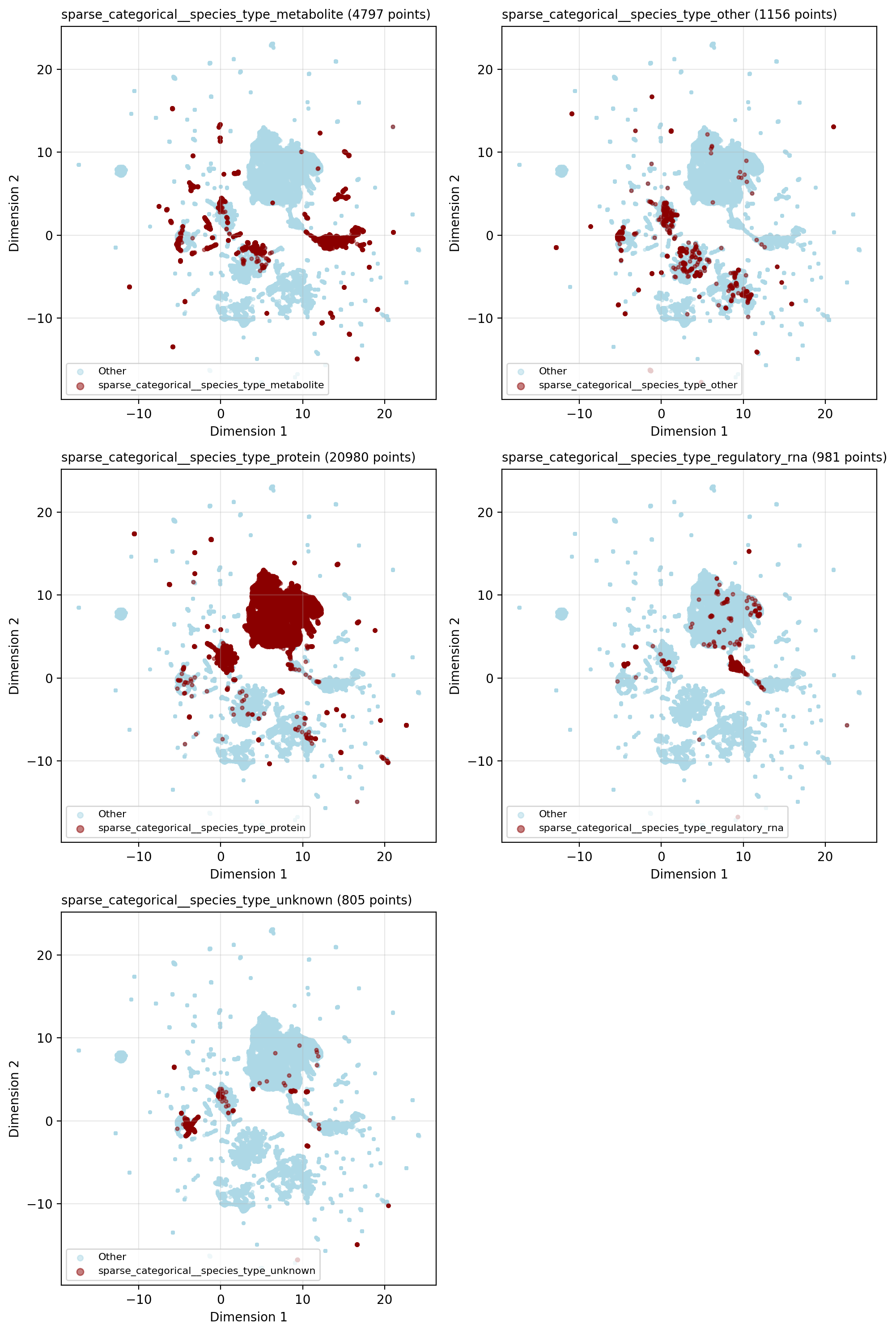
The UMAP visualization shows clear clustering by entity type: proteins cluster with proteins, and metabolites with metabolites. This isn’t surprising given the network’s strong homophily — entities of the same type preferentially connect. STRING alone contributes >80% of the edges in the network, and STRING edges are exclusively protein-protein interactions.

However, entity types don’t completely segregate. Proteins and metabolites intermix at cluster boundaries, and the embedding shows finer-grained structure within each entity type. This suggests the GNN captures more than just entity type — it’s learning the biological organization within these categories. To reveal what additional information the embedding encodes, I will analyze how pathway membership and data source annotations are reflected in the representations

Pathway similarity

To assess pathway organization in the embeddings, I’ll use the comprehensive pathway membership artifact created earlier. This binary tensor encodes both coarse-grained data sources (8 sources) and fine-grained pathway annotations (2800+ Reactome pathways) for each vertex.

For each source and pathway, I’ll calculate the average cosine similarity between all vertex pairs that belong to that category. The fine-grained Reactome pathways are then aggregated to assess whether individual pathways produce tighter clusters than Reactome as a whole.

# not really needed, but we can check artifacts alignments to the canonical vertex and edge feature names from the NapistuData instance
pathway_assignments = comprehensive_pathway_memberships.align_to_napistu_data(napistu_data, inplace=False).data

pathway_similarities = calculate_pathway_similarities(
    embedding_matrix = embeddings,
    pathway_assignments = pathway_assignments[is_species_mask],
    pathway_names = comprehensive_pathway_memberships.feature_names,
)
# rename categories for clarity
pathway_similarities["Reactome (by pathway)"] = pathway_similarities.pop("other")
pathway_similarities["Reactome (overall)"] = pathway_similarities.pop("Reactome")
del pathway_similarities["overall"]

# Sort by value
sorted_items = sorted(pathway_similarities.items(), key=lambda x: x[1])
categories = [item[0] for item in sorted_items]
values = [item[1] for item in sorted_items]

# Create figure and axis
fig, ax = plt.subplots(figsize=(10, 6))

# Create barplot
bars = ax.barh(categories, values, color='steelblue', edgecolor='black', linewidth=0.5)

# Customize the plot
ax.set_xlabel('Within-category cosine similarity', fontsize=12, fontweight='bold')
ax.set_ylabel('Data source', fontsize=12, fontweight='bold')
ax.set_title(
    'Within-category cosine similarity by data source', 
    fontsize=14,
    fontweight='bold',
    pad=20,
    loc='left'
)

# Add value labels on the bars
for i, (cat, val) in enumerate(zip(categories, values)):
    ax.text(val + 0.01, i, f'{val:.3f}', 
            va='center', fontsize=9)

# Add grid for easier reading
ax.grid(axis='x', alpha=0.3, linestyle='--')
ax.set_axisbelow(True)
plt.tight_layout()
plt.show()

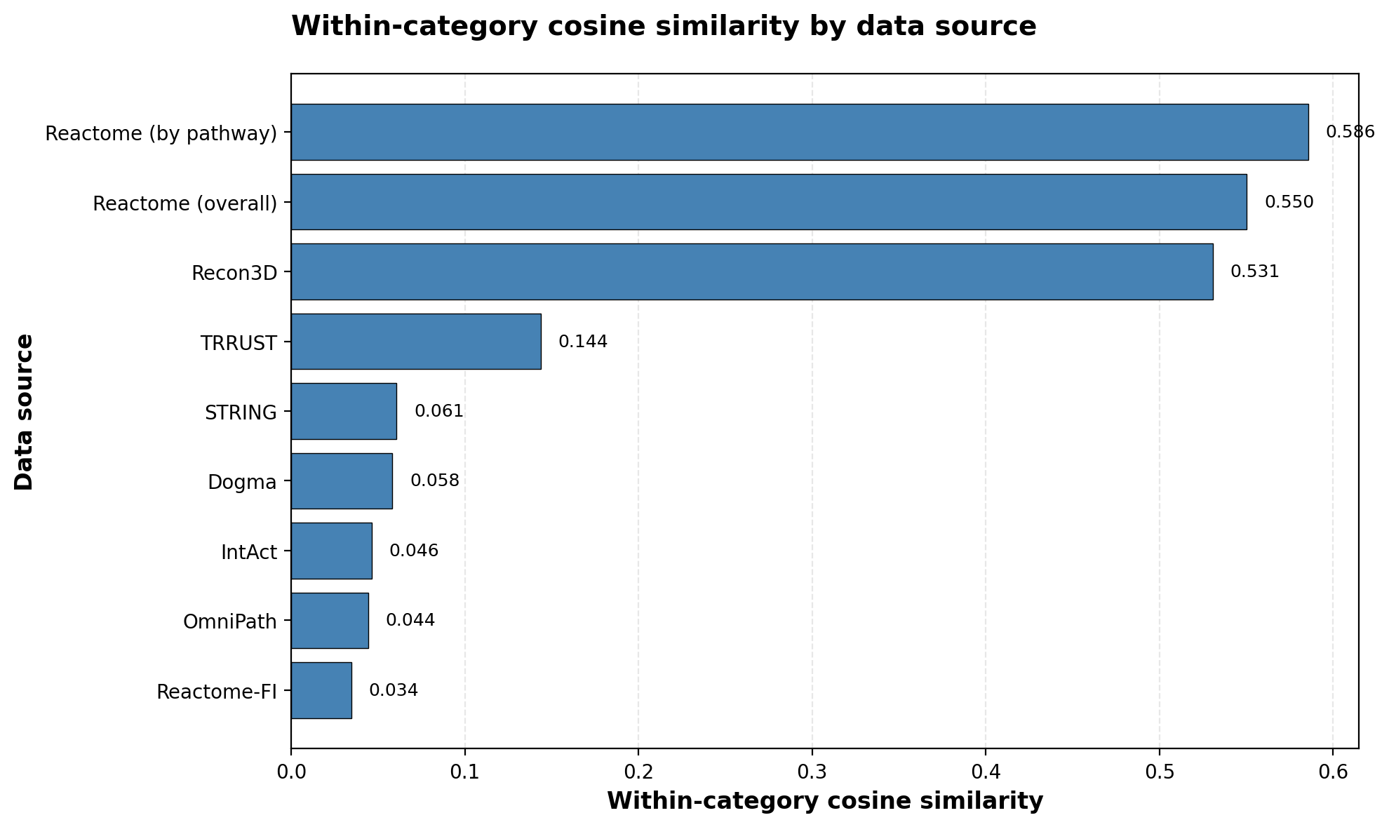
The embedding structure reflects the network’s edge composition. STRING contributes >80% of edges—all protein-protein interactions — which means the training objective is dominated by getting protein relationships right. This pushes the model to spread proteins across the embedding space to capture their diverse interaction patterns, resulting in low within-source similarity for protein-rich databases: STRING (0.061), IntAct (0.046), OmniPath (0.044).

In contrast, specialized sources with fewer, lower-degree entities get pushed into tighter regions of the embedding space. Reactome (0.550 overall, 0.586 by pathway) and Recon3D (0.531) show much higher within-source similarity. These sources contribute distinctive entity types — complexes and proteoforms for Reactome, and detailed metabolic species for Recon3D. The model learns to distinguish these entities from standard proteins. However, because they contribute few edges to the training signal, the model clusters them together rather than resolving fine-grained structure within them.

This explains why Reactome pathways show only modest additional cohesion (0.586) compared to Reactome overall (0.550), the model learns “this is a Reactome entity” but doesn’t strongly differentiate between specific Reactome pathways.

Learned edge weights

Next, I’ll explore what makes a high-confidence edge using sensitivity analysis on the edge encoder.

The edge encoder maps 69 edge attributes to a single weight in (0, 1). To evaluate each attribute’s importance, I calculate its average gradient with respect to the learned edge weight across 1M randomly sampled edges. This sensitivity score reveals which features most strongly influence the model’s confidence in an edge.

device = select_device(mps_valid = True)

top_model = top_model_manager.load_model_from_checkpoint(top_model_manager.best_checkpoint_path)
edge_encoder = get_edge_encoder(top_model)
feature_sensitivities = compute_edge_feature_sensitivity(edge_encoder, napistu_data.edge_attr, 1000000, device)

formatted_feature_sensitivities = format_edge_feature_sensitivity(feature_sensitivities, napistu_data)

fig, ax = plot_edge_feature_sensitivity(formatted_feature_sensitivities, top_n=20, figsize=(16, 8), truncate_names=50)
plt.show()

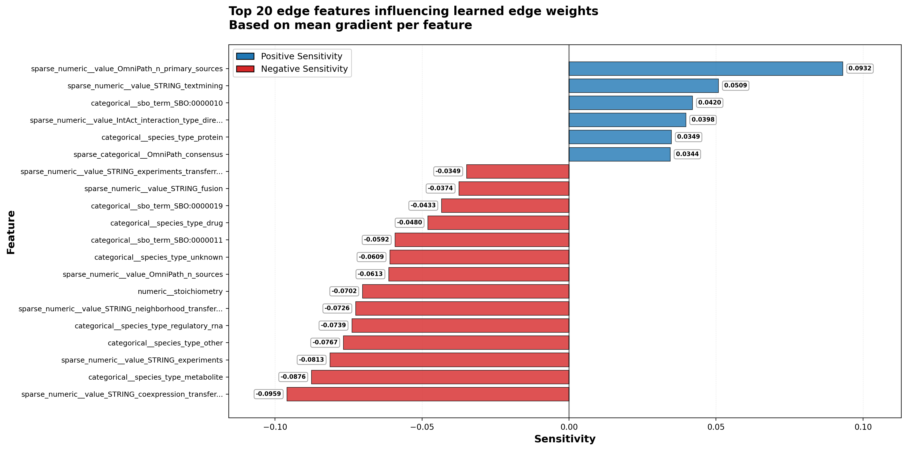
The model shows clear preferences: literature-derived evidence (OmniPath primary sources, STRING text mining) increases edge confidence, while indirect functional evidence (STRING coexpression transfer, experimental transfer) decreases it. This suggests the model may be learning to construct mechanistic regulatory relationships — combinations of physical interactions and functional associations — rather than simply upweighting physical interactions or functional signals independently.

Napistu aims to capture mechanistic relationships at genome-wide scale: an edge from A→B indicates that A is sufficient to modify B (at least in some contexts), enabling paths through the network to represent regulatory cascades. However, our understanding of regulation is highly incomplete. Gold-standard mechanistic resources like Reactome and Recon3D are accurate but sparse — low false positive rates but high false negative rates. To complement them, Napistu integrates broader resources: STRING (primarily functional associations like coexpression) and IntAct/OmniPath (physical interactions like binding and phosphorylation). These provide a dense web of plausible regulatory connections, but conflate mechanistic regulation with its functional byproducts.

The Octopus network thus integrates databases with fundamentally different evidence types. Training on edge prediction across this integrated network may push the model to learn which combinations of features distinguish true mechanistic regulation — relationships that are both physically direct and functionally consequential — from mere functional associations.

The observation that learned edge weights prioritize literature-derived evidence over coexpression is encouraging. It suggests the model may be learning mechanism-grounded causality rather than being misled by correlation.

Interpreting individual features is complicated by the edge encoder’s nonlinear combinations. For example, OmniPath primary sources show strong positive sensitivity while total OmniPath sources show negative sensitivity, suggesting the model values concentrated evidence from specific high-quality sources over diffuse evidence from many sources.

Notably, none of the hand-crafted confidence scores from the original databases — STRING combined score, IntAct MI score, Reactome FI score — appear among the most sensitive features. This suggests the edge encoder is learning data quality signals that differ from expert-designed heuristics, reinforcing the value of end-to-end training for edge weighting.

Finally, I’ll explore the types of edges being predicted by the GraphConv GNN.

Edge predictions

As previously discussed, when negative samples differ too greatly from real edges, the model can exploit vertex attributes that indicate implausible connections, rather than capturing the underlying biological network structure. To address this shortcut, negative samples were generated using the observed node_type strata (i.e., sampling an equal number of species→species, species→reaction, and reaction→species edges as in the real set of edges). Yet, certain vertex features could trivially separate real and negative edges; for instance, regulatory RNAs never interact with metabolites in the dataset

To evaluate whether the model exploits potential misalignment between real edges and negative samples, I’ll compare predicted edge probabilities for each edge class to the probabilities expected from their relative frequencies in real and negative edges

edge_predictions = predict(
    top_model_manager.get_experiment_dict(),
    checkpoint=top_model_manager.best_checkpoint_path
)

species_strata_recovery = summarize_edge_predictions_by_strata(edge_predictions, edge_strata_by_node_species_type)

# Filter to categories with >= 100 edges
species_strata_recovery_filtered = species_strata_recovery[species_strata_recovery['count'] >= 100]

fig, ax = plot_edge_predictions_by_strata(species_strata_recovery_filtered)
plt.show()

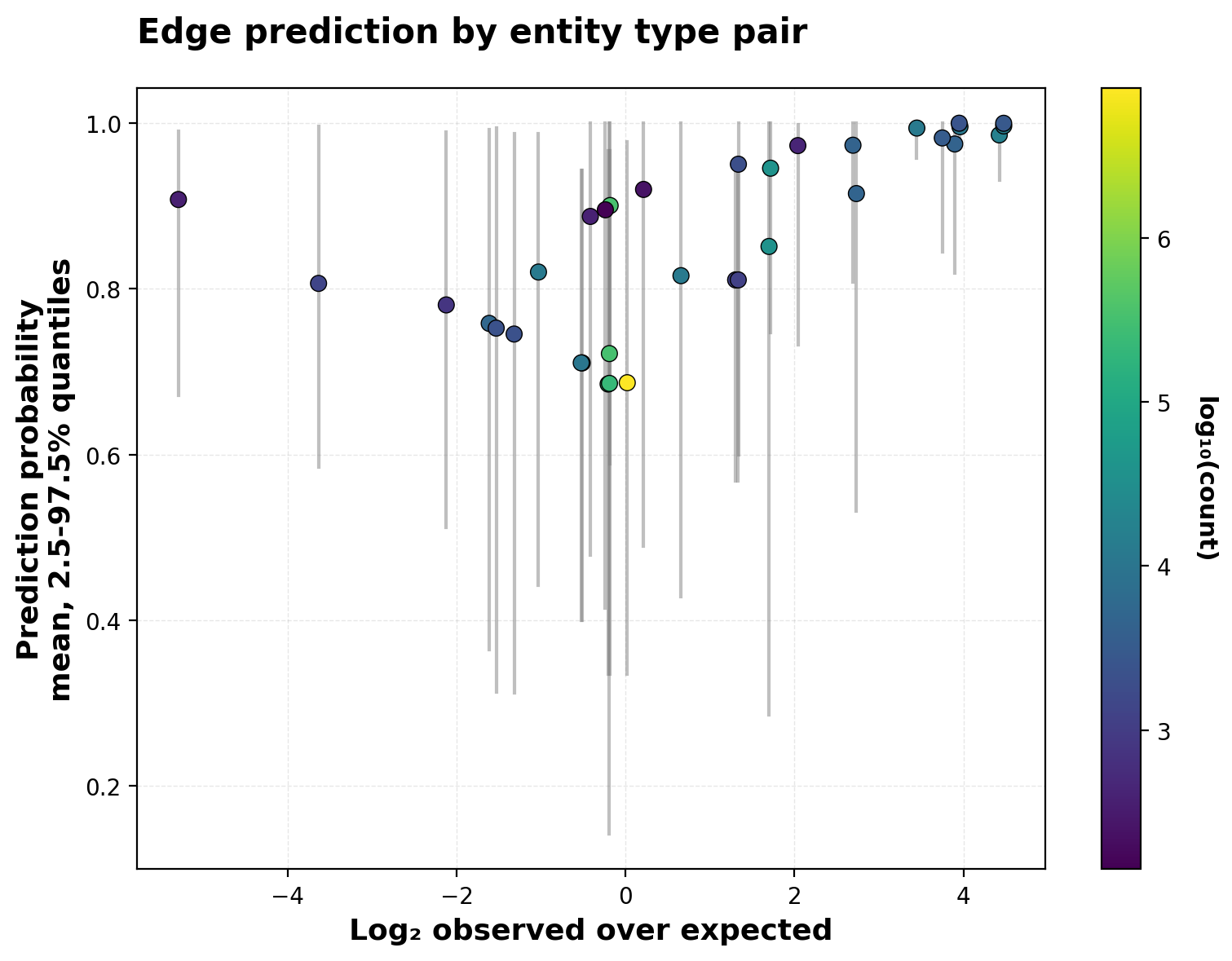
The plot reveals two distinct patterns. For common edge types — particularly protein→protein interactions (bright yellow, log₂ O/E ≈ 0) — real edges and negative samples occur at similar frequencies, yet the model’s predictions span a wide range (0.3-1.0). This indicates the model is learning patterns of vertex similarity that go beyond trivial features like entity type. The model differentiates among protein pairs based on their learned embeddings, not just their shared protein identity.

For rare edge types involving specialized entities (complexes, metabolites from Recon3D), the pattern changes. These categories often show extreme enrichment or depletion (|log₂ O/E| > 2), yet the model assigns them consistently high prediction probabilities regardless of whether they’re enriched or depleted. This likely reflects the tight embedding clusters observed earlier for Reactome and Recon3D entities — specialized molecular species cluster strongly in the embedding space, leading the dot product head to predict high edge probabilities between them even when such edges are rare in the training data.

This analysis suggests the model has learned meaningful biological structure within major edge types while potentially overgeneralizing for rare, specialized entities. The wide prediction spread for protein→protein edges is encouraging for future work, with more expressive heads and validation datasets, these learned similarity patterns could identify novel regulatory connections within well-represented entity types.

Summary

This post introduced Napistu-Torch and demonstrated that training GNNs on genome-scale biological networks is feasible with standard hardware — the complete suite of models trained in ~2 days on a laptop. More importantly, I’ve established the foundational infrastructure needed to explore this space systematically:

• The NapistuDataStore handles conversion from biological networks to PyTorch Geometric format with caching that eliminates rebuild overhead.
• Modular encoders, heads, and edge encoders enable architectural exploration through configuration files rather than code changes.
• PyTorch Lightning integration and CLI-driven workflows make experiments reproducible and trackable via Weights & Biases.
• Edge prediction provides self-supervised training without ground-truth labels while stratified negative sampling maintains computational tractability.
• Vertex embeddings, learned edge weights, and prediction patterns reveal what biological structure the models capture.

The most impactful findings are that different GNN architectures converge on similar biological representations — suggesting the signal is robust—and not trivially recovered from vertex attributes like its data source or molecule type.

This work creates a low-activation-energy foundation for exploring how GNNs can tap the potential of comprehensive biological networks like the Octopus. The hard infrastructure work is done — what remains is the interesting part: using these tools to build accurate genome-scale representations and discover novel biology.