Napistu’s Octopus: An 8-source human consensus pathway model

Introducing the Octopus: Napistu’s eight-source Human Consensus Pathway Model that unites the breadth of protein-protein interaction networks with the depth of regulatory databases and metabolic models.The result is a genome-scale directed graph that is both densely connected and mechanistically precise. In this post, I will:

• Provide an overview of the Octopus model and its construction
• Show side-by-side summaries of individual data sources highlighting their complementarity
• Demonstrate that the model successfully merges results, creating a dense network covering the complete cellular repertoire of genes, metabolites, drugs, and complexes
• Illustrate how source-level information can be carried forward to the Octopus’s graphical network to augment its vertex and edge features

The model is distributed as a set of related Napistu assets bundled together. The core components are two major Napistu data structures:

• SBML_dfs: An in-memory relational database organizing molecular species (genes, metabolites, complexes, drugs) and their relationships (reactions, interactions). I’ll provide a thorough review of this format below.
• NapistuGraph: A directed graph representation of the same network, translating molecular species and reactions into a network optimized for downstream analysis.

Building the 🐙

I built the Octopus using Napistu’s CLI, which processes individual pathway sources, merges them into consensus models, and translates them into genome-scale molecular networks. The build process runs as a cached Quarto notebook — sufficient for present needs, but a dedicated workflow manager like NextFlow or Airflow would be better suited for broader adoption within the research community.

The Octopus build process follows seven sequential steps:

1. Ingest data source-specific content and format as SBML_dfs objects
2. Standardize compartmentalization — the Octopus uses an uncompartmentalized approach for simplicity
3. Merge SBML_dfs objects into a single consensus model
4. Filter cofactors to prevent molecules like water from appearing as hub regulators
5. Convert the SBML_dfs into a NapistuGraph network representation
6. Generate derived summaries including precomputed molecular distances
7. Package all components into a single artifact and deploy to Google Cloud Storage

The uncompartmentalized approach sacrifices one of Napistu’s most compelling features: modeling spatial organization and transport mechanisms. These are fundamental to physiology and pathophysiology — such as proton transport for ATP synthesis or protein aggregation in neurodegeneration. Napistu could uniquely extend quantitative metabolic modeling principles to genome-scale networks of cellular physiology, even treating cell types or tissues as compartments to model local-global process interactions in Systems Physiology.

I’m excited about these directions, but building a compartmentalized model is a major effort — it demands strong biological use cases and high-quality data sources. The biggest challenge is defining the right level of compartmental granularity and aligning data sources to that resolution for effective integration. My current uncompartmentalized approach sidesteps this complexity, though Human Proteome Atlas integration could provide a path forward when the right biological question arises.

Follow Along!

Environment setup

To follow along with the code in this post, you’ll need a Python environment with the napistu package installed. Here’s a simple setup using venv:

1. Install uv (or use pip if preferred)

2. Setup a Python environment:

uv venv --python 3.11
source .venv/bin/activate

# Core dependencies
uv pip install "napistu==0.7.1"
# if you'd like to render the notebook, you'll need to install these additional dependencies
uv pip install seaborn ipykernel nbformat nbclient
python -m ipykernel install --user --name=blog-staging

1. Download the octopus_network.qmd notebook (or copy and paste the relevant code blocks)

2. Configure data_dir in the setup code to a path where you’re comfortable saving the consensus SBML_dfs model

Configuring the Python notebook

import os
from pathlib import Path
import requests
from math import pi

import matplotlib.pyplot as plt
import numpy as np
import pandas as pd
import seaborn as sns

from napistu import utils as napistu_utils
from napistu.gcs import downloads
from napistu import sbml_dfs_utils
from napistu.network import ng_utils
from napistu.sbml_dfs_core import SBML_dfs
from napistu.network.ng_core import NapistuGraph
from napistu.ontologies.constants import SPECIES_TYPE_PLURAL

from shackett_utils.blog.html_utils import display_tabulator

# globals
DATA_DIR = "/tmp/napistu_data"
ASSET = "human_consensus"
VERSION_TAG = "20250923"
INPUT_SBML_DFS_SUMMARIES_URL = "https://raw.githubusercontent.com/shackett/shackett/main/assets/data/octopus_input_sbml_dfs_summaries.json"

# utils
def cooccurrence_to_conditional_prob(cooccur_df):
    set_sizes = np.diag(cooccur_df.values)
    intersection = cooccur_df.values
    conditional_prob = intersection / set_sizes  # P(A|B) = |A ∩ B| / |B|
    return pd.DataFrame(conditional_prob, index=cooccur_df.index, columns=cooccur_df.columns)

def simple_pd_heatmap(df, plot_title, colorbar_label="Counts", fmt="d"):
    # Set up the figure size and style
    plt.rcParams.update({'font.size': 15})  # Base font size
    
    # Create clustermap with proper sizing
    g = sns.clustermap(
        df, 
        annot=True,  # Show values in cells
        cmap='Blues', 
        fmt=fmt,
        cbar_kws={'label': colorbar_label},
        figsize=(12, 10),  # Larger figure
        annot_kws={'size': 12},  # Annotation font size
        cbar_pos=(0.02, 0.83, 0.03, 0.15),  # Colorbar position (left, bottom, width, height)
    )
    
    # Increase font sizes for axis labels
    g.ax_heatmap.set_xlabel(g.ax_heatmap.get_xlabel(), fontsize=14, fontweight='bold')
    g.ax_heatmap.set_ylabel(g.ax_heatmap.get_ylabel(), fontsize=14, fontweight='bold')
    
    # Rotate and adjust tick labels for better readability
    g.ax_heatmap.tick_params(axis='x', labelsize=11, rotation=45)
    g.ax_heatmap.tick_params(axis='y', labelsize=11, rotation=0)
    
    # Add title with proper positioning (left-aligned)
    g.fig.suptitle(plot_title, fontsize=16, fontweight='bold', y=0.98, horizontalalignment='left', x=0.05)
    
    # Adjust layout to prevent clipping
    plt.tight_layout()
    
    # Return the clustermap object for further customization if needed
    return g

def create_pathway_radar_plot(df, figsize=(8, 7), title='Pathway Analysis Radar Plot'):
    
    # Get categories (columns) and pathways (rows)
    categories = list(df.columns)
    pathways = list(df.index)
    
    # Number of variables
    num_vars = len(categories)
    
    # Compute angle for each axis
    angles = [n / float(num_vars) * 2 * pi for n in range(num_vars)]
    angles += angles[:1]  # Complete the circle
    
    # Initialize the plot
    fig, ax = plt.subplots(figsize=figsize, subplot_kw=dict(projection='polar'))
    
    # Color palette for different pathways
    colors = plt.cm.tab10(np.linspace(0, 1, len(pathways)))
    
    # Plot each pathway
    for idx, pathway in enumerate(pathways):
        values = df.loc[pathway].values.astype(float)
        
        # Log10 transform (add 1 to avoid log(0))
        log_values = np.log10(values + 1)
        
        # Complete the circle
        plot_values = list(log_values) + [log_values[0]]
        
        # Plot
        ax.plot(angles, plot_values, 'o-', linewidth=2, 
                label=pathway, color=colors[idx], alpha=0.7)
        ax.fill(angles, plot_values, alpha=0.15, color=colors[idx])
    
    # Fix axis to go in the right order and start at 12 o'clock
    ax.set_theta_offset(pi / 2)
    ax.set_theta_direction(-1)
    
    # Set category labels - use built-in matplotlib positioning
    ax.set_xticks(angles[:-1])
    ax.set_xticklabels(categories, size=11)
    
    # Adjust label padding to move them outside the plot
    ax.tick_params(axis='x', pad=20)
    
    # Set y-axis labels to show original values at powers of 10
    # Determine the max value to set appropriate range
    max_log_value = np.max(np.log10(df.values.astype(float) + 1))
    
    # Create ticks at powers of 10: 10, 100, 1000, 10000, etc.
    max_power = int(np.ceil(max_log_value))
    ytick_values = [10**i for i in range(1, max_power + 1)]
    ytick_positions = [np.log10(v + 1) for v in ytick_values]
    
    ax.set_yticks(ytick_positions)
    ax.set_yticklabels([f'{v:,}' for v in ytick_values], size=9)
    ax.set_ylim(0, np.log10(10**max_power + 1))
    
    # Add grid
    ax.grid(True, linestyle='--', alpha=0.7)
    
    # Add legend
    plt.legend(loc='upper right', bbox_to_anchor=(1.3, 1.1), fontsize=10)
    
    # Add title
    plt.title(title, size=16, pad=20)
    
    plt.tight_layout()
    
    return fig, ax

Data sources

The Octopus’s integration success stems from Napistu’s flexible SBML_dfs data structure, which standardizes diverse pathway sources while preserving their unique molecular and mechanistic contributions.

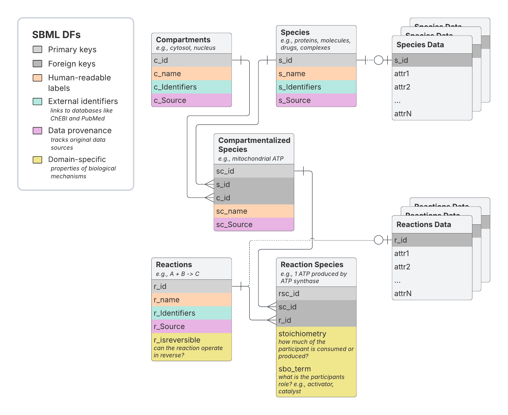
Overview of the SBML_dfs pathway representation

The core SBML_dfs data representation involves five tables linked by primary key-foreign key relationships:

• Compartments: Define distinct cellular locations (e.g., cytosol, nucleoplasm). Uncompartmentalized models contain only “cellular component” by convention.
• Species: Catalog distinct molecular entities including proteins, metabolites, complexes, and drugs.
• Compartmentalized Species: Map each species to its specific compartmental locations.
• Reactions: Represent distinct biochemical events including metabolic reactions, complex formation, and physical/functional interactions.
• Reaction Species: Define each compartmentalized species’ role in specific reactions (substrate, catalyst, inhibitor, etc.).

Additional optional tables store quantitative annotations beyond the core schema:

• Species Data: Contains tables with molecular species-specific quantitative attributes.
• Reactions Data: Contains tables with reaction-specific quantitative attributes.

Source descriptions

Each data source is formatted as a separate SBML_dfs object encapsulating its molecular species, their interactions, and any quantitative data.

• Reactome is the human gold-standard pathway database, employing rigorous expert curation with multi-tier review by over 820 scientists to produce reaction-centric models of cellular processes.
• Recon3D is a comprehensive human metabolic model that enables quantitative flux balance analysis and phenotype prediction.
• STRING is a comprehensive protein interaction database that integrates evidence from seven distinct channels with probabilistic scoring to capture functional associations rather than directional causality. Its strength is broad multi-organism coverage with confidence scores calibrated to known pathway relationships.
• IntAct is a manually curated database of experimentally verified molecular interactions with unprecedented annotation depth, making it the gold standard for high-confidence molecular interaction data.
• Reactome-FI transforms Reactome’s detailed biochemical reactions into simplified functional interaction networks using machine learning.
• OmniPath is a comprehensive integration database that combines data from over 100 resources into unified directed signaling networks with sophisticated consensus-building mechanisms. It specializes in literature-curated activity flow interactions with effect signs (activation/inhibition).
• TRRUST uses sentence-based text mining to identify transcription factor-target regulatory relationsh1ips from Medline abstracts.
• Dogma is a Napistu-specific resource that contributes gene annotations to help merge species across different primary ontologies without adding reactions to the consensus model.

Source comparisons

To understand how these sources complement each other, I’ll provide four side-by-side analyses examining the scale and characteristics of each database:

• Scale: How many species and reactions does each source contain?
• Molecular diversity: What types of entities exist (proteins, metabolites, complexes, drugs)?
• Interaction mechanisms: How do molecules connect (undirected associations, directed regulation, metabolic transformations)?
• Quantitative data: What additional measurements do sources provide (confidence scores, expression levels, binding affinities)?

These comparisons use summary statistics extracted from each source’s SBML_dfs during the Octopus build process. The summaries were saved to a public GitHub repository for reproducibility and transparency. For reference, the source summaries were generated using this non-runnable code block:

from napistu import consensus
from napistu.sbml_dfs_core import SBML_dfs
from napistu import utils

sbml_dfs_uris = [
    # mechanisms
    "napistu_data/human_consensus/cache/reactome/reactome.pkl",
    "napistu_data/human_consensus/cache/bigg.pkl",
    # consensus interactions
    "napistu_data/human_consensus/cache/hpa_filtered_string.pkl",
    # PPIs
    "napistu_data/human_consensus/cache/intact.pkl",
    # regulatory mechanisms
    "napistu_data/human_consensus/cache/omnipath.pkl",
    "napistu_data/human_consensus/cache/reactome_fi.pkl",
    "napistu_data/human_consensus/cache/trrust.pkl",
    # gene annotations
    "napistu_data/human_consensus/cache/dogma_sbml_dfs.pkl",
]

sbml_dfs_list = [SBML_dfs.from_pickle(uri) for uri in sbml_dfs_uris]

# reorganize as a list and table containing model-level metadata from the individual SBML_dfs
sbml_dfs_dict, pw_index = consensus.prepare_consensus_model(sbml_dfs_list)
sbml_dfs_dict_summaries = {k: v.get_summary() for k, v in sbml_dfs_dict.items()}
utils.save_json("<<MY_LOCAL_PATH>>/input_sbml_dfs_summaries.json", sbml_dfs_dict_summaries)

I can load these pre-computed summaries directly from GitHub:

sbml_dfs_dict_summaries = requests.get(INPUT_SBML_DFS_SUMMARIES_URL).json()

These summaries enable direct side-by-side comparison of each source’s unique characteristics and contributions to the consensus model.

Scale

I’ll count entities in each source to assess their relative sizes.

# load the SBML_dfs' summaries from GitHub
entity_type_counts = (
    pd.DataFrame({k: v["n_entity_types"] for k, v in sbml_dfs_dict_summaries.items()})
    .T
    .sort_index(axis = 1)
)

display_tabulator(entity_type_counts, layout = "fitDataTable", caption = "Entity counts per source")

Entity counts per source

Sources contain similar numbers of molecular species but reaction counts vary dramatically — from TRRUST’s ~8K reactions to STRING’s 4.2M. Dogma contains only one placeholder reaction since it contributes gene annotations rather than interactions, helping merge species across different ontologies (Ensembl, UniProt, Entrez).

Molecular diversity

Each source specializes in different molecular entity types based on their ontological annotations.

species_type_counts = (
    pd.DataFrame({k: v["n_species_per_type"] for k, v in sbml_dfs_dict_summaries.items()})
    .astype('Int64')
    .fillna(0)
    .T
    .sort_index(axis = 1)
    .rename(columns = SPECIES_TYPE_PLURAL)
)
display_tabulator(
  species_type_counts,
  layout = "fitDataTable",
  caption = "Counts of molecular species types in each source"
)

RADAR_ORDER = ["proteins", "metabolites", "drugs", "unknowns", "other", "regulatory RNAs", "complexes"]
fig, ax = create_pathway_radar_plot(
    species_type_counts[RADAR_ORDER],
    title = "Species types by pathway source",
)
plt.show()

Counts of molecular species types in each source

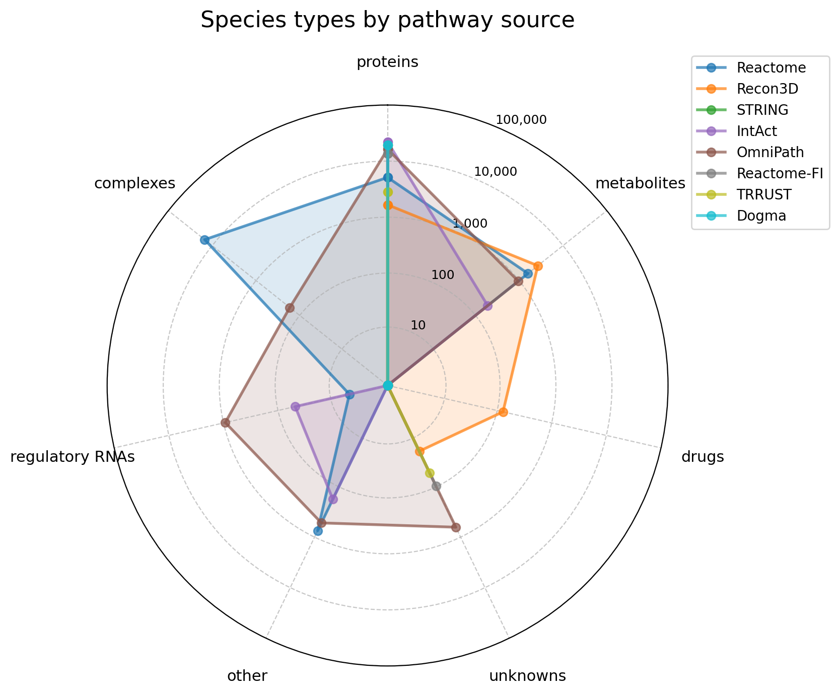
Clear specialization patterns emerge: gene-centric sources (STRING, Dogma, Reactome-FI, TRRUST), metabolite-focused databases (BiGG), and comprehensive resources covering diverse molecular species (Reactome, IntAct, OmniPath).

Interaction mechanisms

I’ll examine interaction types using Systems Biology Ontology (SBO) terms that define molecular roles:

• Interactor: Undirected associations
• Stimulator/Inhibitor/Modifier: Regulators of expression or activity
• Modified: Targets of regulation
• Catalyst: Enzymes and transporters
• Substrate/Product: Consumed or produced molecules

sbo_term_counts = (
    pd.DataFrame({k: v["sbo_name_counts"] for k, v in sbml_dfs_dict_summaries.items()})
    .astype('Int64')
    .fillna(0)
    .T
    .sort_index(axis = 1)
)
display_tabulator(
    sbo_term_counts,
    width="auto",
    layout="fitDataStretch",
    caption = "Counts of reaction participant roles in each source"
)

RADAR_ORDER = ["catalyst", "reactant", "product", "stimulator", "inhibitor", "modifier", "modified", "interactor"]
fig, ax = create_pathway_radar_plot(
    sbo_term_counts[RADAR_ORDER],
    title = "SBO terms by pathway source",
    )
plt.show()

Counts of reaction participant roles in each source

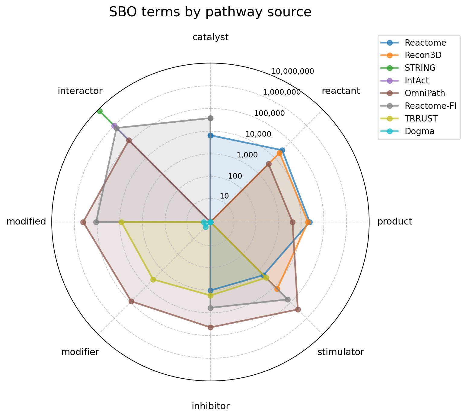
Broad sources like STRING favor generic “interactor” classifications, while specialized databases like Recon3D and Reactome capture specific mechanistic detail more faithfully.

Quantitative data

Beyond structural information, sources provide additional annotations and metadata for both molecular species and their interactions.

data_summaries = {k: v["data_summary"] for k, v in sbml_dfs_dict_summaries.items() if len(v["data_summary"]["reactions"]) > 0}

data_summaries_list = []
for k, v in data_summaries.items():
    for entity_type, entity_data in v.items():
        if len(entity_data) > 0:
            for table_name, table_data in entity_data.items():
                table_summary ={
                    "table_name" : table_name,
                    "entity_type" : entity_type,
                    "n_rows" : table_data["n_rows"],
                    "columns" : ", ".join(table_data["columns"]),
                }
                data_summaries_list.append(table_summary)
data_summaries_df = pd.DataFrame(data_summaries_list)

display_tabulator(
    data_summaries_df,
    wrap_columns = "columns",
    column_widths = {"columns" : "65%"},
    caption = "Additional species- and/or reactions-data in each source"
)

Additional species- and/or reactions-data in each source

This additional data falls into two key categories: confidence scoring systems (STRING interaction scores, IntAct experimental evidence) and mechanistic granularity (OmniPath activation/inhibition breakdowns, IntAct interaction types). Both provide crucial context for assessing interaction reliability and biological mechanisms.

Source compatibility

Many data sources used by Napistu, like STRING and OmniPath, already aim to integrate multiple upstream data sources into a consistent consensus. Napistu builds on these resources to merge what would otherwise be incompatible data sources into a single, well-mixed model. Without proper integration, sources would separate like oil and water — each forming disconnected subnetworks with minimal overlap. Instead, we need to gel them together by establishing a unified molecular vocabulary that enables seamless integration of source-specific interactions.

Napistu accomplishes this integration through:

• Data standardization: Systematic identifiers and SBO ontology terms create a common vocabulary for describing molecules and their interactions across diverse sources
• Algorithmic merging: A consensus procedure that identifies equivalent entities and reconciles overlapping information into a single integrated model

Merging SBML_dfs objects into a consensus SBML_dfs

Merging multiple SBML_dfs objects into a consensus model requires resolving entities by determining which compartments, species, and reactions are shared across sources. This process works through tables in logical order (compartments & species $\rightarrow$ compartmentalized species $\rightarrow$ reactions & reaction species), aggregating a single table drawn from all models to construct:

• Consensus tables: New unified tables with standardized structure
• Key mapping tables: Lookup tables linking old source-specific primary keys to new consensus keys for updating foreign key relationships

Two variables are critical for successful merging:

• Identifiers: Determine what can be merged by organizing systematic identifiers as curated lists, each defined by ontology, identifier, and bioqualifier (e.g., “BQB_IS” or “BQB_HAS_PART”)
• Sources: Track what has been merged by associating each consensus entity with all contributing data sources

The consensus algorithm proceeds through four steps:

1. Resolve foundational entities: Use greedy network-based matching to identify species and compartments through shared identifiers, connecting entities that share BQB-coded systematic identifiers
2. Define compartmentalized species: Map resolved species to their appropriate compartmental locations
3. Merge reactions: Update reaction species annotations and identify redundant reactions based on participants and mechanisms
4. Harmonize data tables: Update species_data and reactions_data with consensus primary keys, aggregating results to ensure one row per consensus entity

The consensus algorithm is robust but exposes incompatibilities between models when sources use different ontologies or resolution levels. If compartments are defined at different granularities or species use incompatible identifier systems, sources merge poorly — essentially speaking different languages. Rather than combining, as intended, they produce networks with multiple disconnected subgraphs that negate the benefits of consensus modeling. Many incompatibilities can be identified during the preprocessing stage through schema validation and syntactic checks. However, additional conflicts often emerge only during post-consensus validation, which evaluates whether molecular species—and, where applicable, reactions—have been accurately and semantically merged across heterogeneous sources.

Loading the 🐙

With the consensus algorithm framework established, let’s examine the actual eight-source Octopus model to see how well these theoretical merging principles work in practice. To do this, I’ll download the pre-built model from Google Cloud Storage and provide some quick summaries of its core properties.

The Octopus network is available through GCS and gets updated periodically as sources are added and Napistu data structures evolve. To ensure reproducibility for this post and others like Network Biology with Napistu, Part 2: Translating Statistical Associations into Biological Mechanisms, tagged versions are preserved for reliable future access. Here, I’ll load a tagged version compatible with Napistu 0.7.1.

This represents the latest human consensus model as of October 2025, but the model continues advancing (hopefully toward a 10-source 🦑 model soon!). To access the most current version, simply install the latest Napistu release and remove the version tag from gcs.downloads.load_public_napistu_asset.

# ~3 min load
# download and cache the Octopus sbml_dfs and the other assets its bundled with
sbml_dfs_path = downloads.load_public_napistu_asset(
    asset = ASSET,
    subasset = "sbml_dfs",
    data_dir = DATA_DIR,
    # download the tagged version for reproducibility and Python env compatibility
    version = VERSION_TAG,
)

sbml_dfs = SBML_dfs.from_pickle(sbml_dfs_path)

🐙 summary

With the core SBML_dfs object loaded, I’ll examine its high-level properties using the show_summary method.

summary_stats = sbml_dfs.get_summary()
summary_table = sbml_dfs_utils.format_sbml_dfs_summary(summary_stats)
display_tabulator(
    summary_table,
    width="auto",
    layout="fitDataStretch",
    caption = "Consensus SBML_dfs summaries"
)

Consensus SBML_dfs summaries

The consensus model contains genes/proteins, metabolites, complexes, drugs, and regulatory RNAs within a single compartment — cellular component (the root term of GO’s cellular component category). The model encompasses approximately 4.5M reactions spanning undirected interactions, directed regulation, and complex multi-participant regulatory mechanisms.

While the earlier source comparisons demonstrated each database’s potential contributions, the key question remains: did the sources actually merge into a single well-mixed model? Successful integration requires extensive molecular species sharing across sources and meaningful reaction overlap. Rather than separate, highly connected subnetworks with minimal inter-source connections, we want a unified network where sources are genuinely integrated.

The model’s Source objects provide the answer — they track which data sources contributed to each species, compartment, and reaction, enabling direct assessment of integration success.

Shared molecular vocabulary

To assess integration success, I’ll examine which data sources contributed to each molecular species through contingency tables of species-source occurrences. Values reflect how many of a source’s molecular species merged into each consensus species — typically 0 (not present) or 1 (exact match), though occasionally higher when multiple protein annotations roll up to a single gene.

species_source_occurrence = sbml_dfs.get_source_occurrence("species")
display_tabulator(
    species_source_occurrence.head(),
    layout = "fitDataTable",
    caption = "Example molecular species and the sources they were originally found in"
)

Example molecular species and the sources they were originally found in

I can visualize species sharing patterns by converting the occurrence matrix ($X$) into a cooccurrence matrix ($C$) using:

\[C = B B^T\]

Where $B = \mathbf{1}(X \neq 0)$ is the binary matrix obtained by converting non-zero entries of $X$ to 1.

species_source_cooccurrence = (
    sbml_dfs.get_source_cooccurrence("species")
    .rename_axis('Database', axis=0)
    .rename_axis('Database', axis=1)
)

simple_pd_heatmap(species_source_cooccurrence, "Species Source Co-Occurrence")

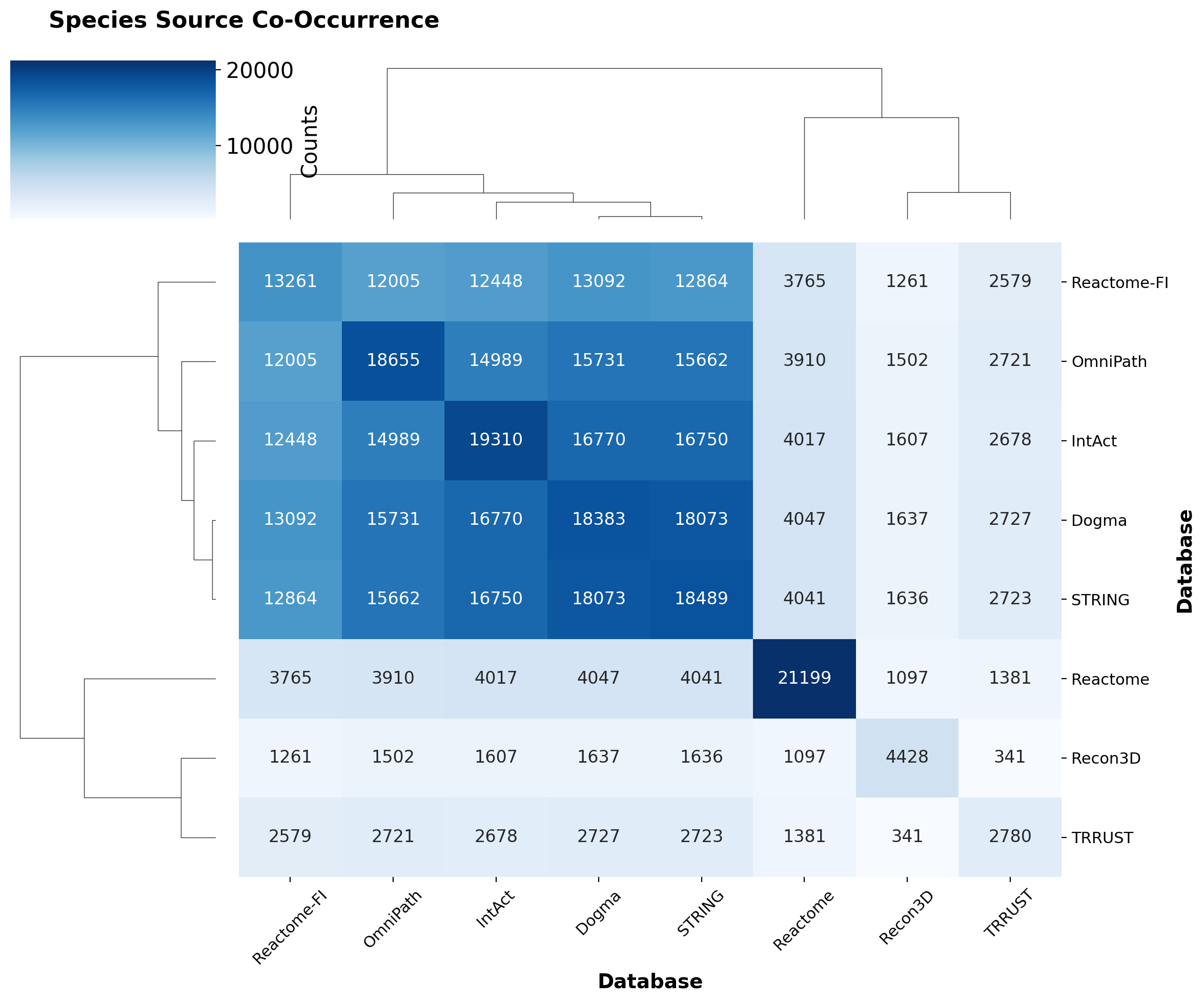
The heatmap reveals that gene-centric, dense sources (STRING, Dogma, Reactome-FI) cluster together with similar molecular coverage, while Reactome, Recon3D, and TRRUST remain more isolated. This reflects TRRUST’s smaller size and the molecular specialization of Reactome and Recon3D compared to comprehensive protein databases.

To quantify this specialization, I’ll identify species unique to individual sources.

private_species = species_source_occurrence.loc[(species_source_occurrence != 0).sum(axis=1) == 1]

private_species_source_counts = (
    (private_species != 0)
    .sum()
    .sort_values(ascending=False)
    .rename("Private species")
    .to_frame()
    .T
)

display_tabulator(
    private_species_source_counts,
    width="auto",
    layout="fitDataStretch",
    include_index=False,
    caption = "Private molecular species from each source"
)

Private molecular species from each source

Several sources contribute substantial numbers of private species, each for logical reasons:

• Reactome: Detailed complex mechanisms with fine-grained complex definitions
• OmniPath: Extensive drug collections (PubChem) and microRNAs (MirBase)
• IntAct: Small molecules and microRNAs alongside core protein interactions
• Recon3D: Extensive coverage of metabolites and lipids

The Octopus successfully integrates molecular species, with proteins shared across multiple sources while specialized molecular types arise from domain-specific resources.

Reaction overlap reveals data source specialization

To understand what individual sources contribute, I’ll analyze reaction source occurrences and cooccurrences using a similar approach to species analysis.

To interpret this analysis, readers should understand two important points:

• Strict merging criteria: Reactions merge only with identical participants and SBO terms. A reaction between genes A and B won’t merge if one source labels them inhibitor $\rightarrow$ modified while another uses modifier $\rightarrow$ modified, explaining the low overlap we’ll observe.
• Analysis scope: This analysis excludes interactor-interactor interactions because the existing tooling is designed to surface information relevant for graph construction, where these interactions become direct edges between molecular species with no reaction vertices added.

reactions_source_occurrence = sbml_dfs.get_source_occurrence("reactions")

display_tabulator(
    reactions_source_occurrence.head(),
    width="auto",
    layout="fitDataStretch",
    caption = "Example reactions and the sources they were originally found in"
)

Example reactions and the sources they were originally found in

The reaction occurrence data is notably sparse, and the order-of-magnitude differences in reaction counts between sources complicate direct cooccurrence visualization.

To better assess source dependencies, I’ll calculate conditional probabilities $\Pr(A|B)$ from the cooccurrence matrix, showing how likely a reaction from source $B$ also appears in source $A$.

reactions_source_cooccurrence = (
    sbml_dfs.get_source_cooccurrence("reactions")
    .rename_axis('Database', axis=0)
    .rename_axis('Database', axis=1)
)

reactions_source_conditional_prob = cooccurrence_to_conditional_prob(reactions_source_cooccurrence)

simple_pd_heatmap(reactions_source_conditional_prob, "Conditional probability of reaction found in column source\n given that it occurs in the row source", fmt=".3f", colorbar_label="Probability")

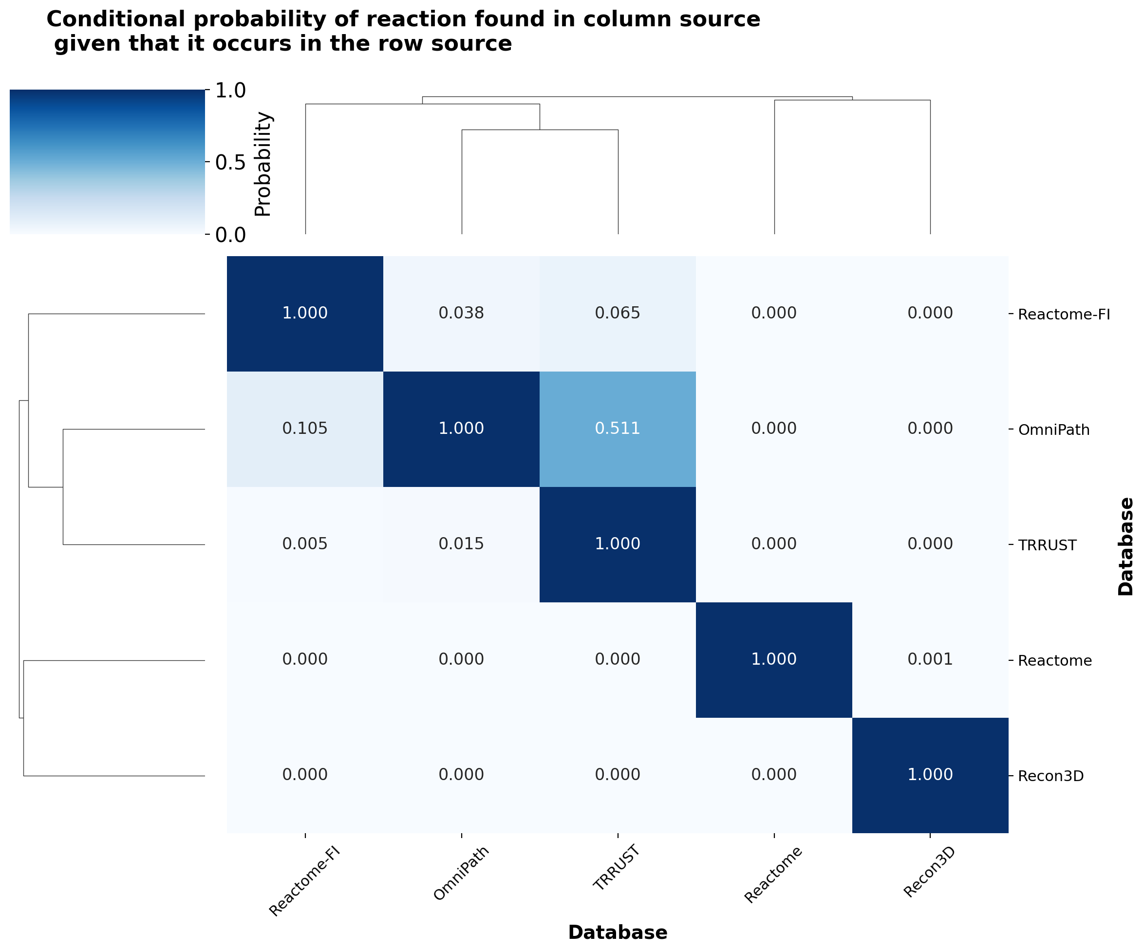
The conditional probability analysis reveals distinct patterns: Reactome and Recon3D reactions remain largely unique, while meaningful overlap exists between Reactome-FI, OmniPath, and TRRUST. The strongest overlap occurs between TRRUST and OmniPath (50% of TRRUST interactions also appear in OmniPath) — an expected result since TRRUST is one of the resources incorporated into OmniPath.

These patterns demonstrate successful species integration alongside preserved source-specific reaction diversity, with each database contributing substantial unique mechanistic content to the consensus model.

Decorating the 🐙 graph with species and reaction data

While SBML_dfs comprehensively organizes pathway data, network analyses like personalized PageRank require graph representations. NapistuGraphs convert this tabular data into networks where compartmentalized species and reactions become vertices connected by information flow edges. Built on igraph’s foundation, they combine versatile graph operations with biological annotations, data provenance, and specialized network biology methods.

A NapistuGraph was bundled with the SBML_dfs downloaded above, enabling direct loading and analysis:

napistu_graph_path = downloads.load_public_napistu_asset(
    asset = ASSET,
    subasset = "napistu_graph",
    data_dir = DATA_DIR,
    version = VERSION_TAG
)

napistu_graph = NapistuGraph.from_pickle(napistu_graph_path)

summary_stats = napistu_graph.get_summary()
summary_table = ng_utils.format_napistu_graph_summary(summary_stats)
display_tabulator(
    summary_table,
    wrap_columns = True,
    column_widths = {"Value" : "80%"},
    caption = "Summaries of the NapistuGraph network"
)

Summaries of the NapistuGraph network

Many vertex and edge attributes mirror those from the SBML_dfs summaries.

The critical quantitative attribute is edge weight, representing each interaction’s plausibility and strength. Edge weights drive most graph algorithms — from shortest path calculations and network layouts to propagation methods. However, capturing this complexity in a single attribute becomes increasingly challenging as more sources contribute quantitative information relevant to regulatory plausibility.

Earlier versions of the Napistu human consensus model used simple heuristics for edge weighting: assign favorable (low) weights to sparse mechanistic sources like Reactome while quantitatively weighting STRING based on its confidence scores. This approach worked when STRING dominated the quantitative landscape, but the Octopus model’s addition of moderately dense sources — OmniPath, IntAct, and Reactome-FI — each with their own confidence metrics complicates this strategy. Rather than continuing to stack ad hoc weighting schemes, the growing diversity of quantitative evidence calls for more principled approaches.

I’m increasingly interested in learning edge trustworthiness empirically through predictive performance rather than manual calibration. While this is challenging for biological applications like regulatory network prediction due to limited ground truth data, the network itself offers opportunities for self-supervised learning. However, realizing this potential requires a rich feature space beyond basic topological properties — which brings us to the wealth of quantitative information that can be integrated into the NapistuGraph representation.

The default NapistuGraph contains a limited array of vertex and edge attributes, but there’s actually a wealth of quantitative information highlighted throughout this post that can be integrated directly into the Octopus network. The power of Napistu’s design becomes apparent when we start layering in this additional context. I’ll demonstrate by augmenting the graph with two particularly valuable information types:

• add_sbml_dfs_summaries: Generates source and ontology occurrence data for all vertices, revealing which databases contributed to each node and what biological categories they represent
• add_all_entity_data: Transfers comprehensive quantitative measurements from reactions_data and species_data tables directly onto their corresponding edges and vertices

# augment the graph
# add ontology and source data to vertices
napistu_graph.add_sbml_dfs_summaries(sbml_dfs, stratify_by_bqb = False)

# add reactions_data to edges
napistu_graph.add_all_entity_data(sbml_dfs, "reactions", overwrite=True)
napistu_graph.add_all_entity_data(sbml_dfs, "species", mode = "extend")

summary_stats = napistu_graph.get_summary()
summary_table = ng_utils.format_napistu_graph_summary(summary_stats)
display_tabulator(
    summary_table,
    wrap_columns = True,
    column_widths = {"Value" : "80%"},
    caption = "Post-augmentation summaries of the `NapistuGraph` network"
)

Post-augmentation summaries of the `NapistuGraph` network

Now, we’ve gone from a relatively spartan set of vertex and edge attributes to a comprehensive graph of human cellular physiology enriched with detailed biological annotations that describe what each vertex and edge represents. This is a robust foundation for training expressive network-based methods like graph neural networks.

Summary

The Octopus model integrates eight diverse pathway databases into a unified, genome-scale network of human cellular physiology. Through systematic merging of complementary data sources, the model establishes a shared molecular vocabulary while preserving each source’s specialized contributions:

• Molecular species integration: Proteins and other species are effectively shared across sources, creating a common parts list that specialized databases can extend with domain-specific molecules (metabolites from Recon3D, complexes from Reactome).
• Reaction specialization: Sources show modest but meaningful overlap in reactions, with each database contributing unique mechanisms that reflect its individual curation focus.

The resulting NapistuGraph provides a framework for layering extensive biological information onto network structures. Source provenance, confidence scores, ontological classifications, and mechanistic annotations can be systematically integrated as vertex and edge attributes, enabling sophisticated analyses from network propagation to machine learning approaches.

The Octopus model is now ready for use. I’m excited to build on this foundation and to see how the community engages with this new resource.