

Flattening the Gompertz Distribution
In this post I’ll explore the Gompertz law of mortality which describes individuals’ accelerating risk of death with age.
The Gompertz equation describes per-year hazard (i.e., the likelihood of surviving from time $t$ to $t+1$) as the product of age-independent parameter $\alpha$ and an age-dependent component which increases exponentially with time scaled by another parameter $beta$ ($e^{\beta \cdot t}$).
The equation is thus:
\[\large h(t) = \alpha \cdot e^{\beta \cdot t}\]The Gompertz equation is often studied by taking its natural log resulting in a linear relationship between log(hazard) and increasing risk with age.
\[\large \ln(h(t)) = \ln(\alpha) + \beta \cdot t\]Formulating and estimating the parameters of demographic hazard models like the Gompertz’s equation is an active area of research, and there is a lot of information out there catering to both the academic and lay audiences. Still, when reviewing this literature, I did not see a clear summary of how decreases in $\beta$ (the chief aim of longevity research) would lead to lifespan extension.
For me, this is one of the most interesting properties of the Gompertz model, and this potential has been touted by my colleagues Graham Ruby and Eugene Melamud at Calico for some time.
Here, I’ll focus on a quantitative treatment of two related questions related to the potential of lifespan extension through slowing aging:
- How was the lifespan extension seen across the $20^{th}$ borne out in changes in baseline mortality ($\alpha$)? The 1.9-fold lifespan extension across the century was borne-out through a 26-fold decrease in baseline mortality ($\alpha$).
- What would life expectancy be if there were a comparable decrease in $\beta$? A 26-fold decrease in $\beta$ would extend human life expectancy to around 1,000 years.
I am NOT an expert on demographic models, so through ignorance (but also conveniently for brevity!) I’ll be leaving out lots of relevant information.
Additionally, while I am a current Calico employee, I want to emphasize that this and any other posts on my personal blog are my personal thoughts and do not necessarily reflect the opinions of my employer.
Background
Life Tables
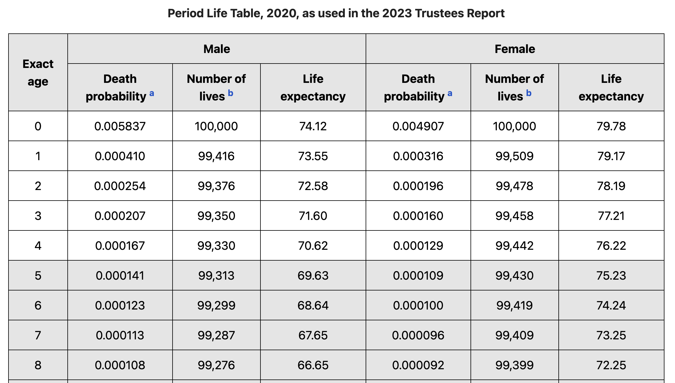
Demographic models of mortality and life expectancy are built from “life tables.” Life tables contain both the number of individual of a given age that are living in the selected year, and the number of deaths that occurred in these ages during the selected year. This is sufficient to calculate the probability of an individual of a given age dying that year (i.e., the hazard).
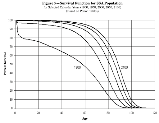
Life tables can either be “period” life tables which describe the mortality of a population within a narrow window of time, while “cohort” life tables describe the mortality of a cohort of individual born within a narrow window of time. In this post I’ll be focusing on period life tables, which can be obtained from many sources, for example here is an example from the social security administration.
The Origin of Life Tables
As mentioned above, creating life tables requires (1) the number of individuals at each age, and (2) the number of deaths at each age. The easiest way to accomplish (1) is through a census, while (2) requires solid record keeping. These conditions were rarely in place at the same time so early life tables were derived from birth and death records rather than direct summaries of demographics.
In 1693 the British astronomer Edmon Halley studied the birth and death records of the city of Breslau. Breslau happened to be in a steady-state where the number of births approximately equaled the number of deaths. He used this information to create the first life table describing the distribution of residents’ ages. Using this information, Halley demonstrated how to price annuities leading to the birth of Actuarial Science.
Around 1750, the Swiss mathematician Leonard Euler re-derived the work of Halley while exploring the exponential growth of populations. His formulation of exponential growth allowed life tables to be generated for non-stationary populations.
With proper censuses it is now easier to just plug in measured values into a life table, but the lack of this information produced elegant math for describing population dynamics amid indirect measurements. These continue to be fundamental for studying both evolutionary and ecological dynamics.
Gompertz’s Law
Nearly 200 years ago, Benjamin Gompertz, a British actuary, described the mortality of populations in a life table (i.e., the survival curve) as a symmetrical sigmoidal function. Because the function is sigmoidal it indicates that the absolute mortality peaks at the average lifespan; past this point, while relative mortality increases the lower number of individuals remaining results in fewer total deaths.
Later, the modern Gompertz law of mortality was derived from the more general Gompertz equation. Unlike the sigmoidal formulation, the Gompertz law focuses on relative mortality hence risk continues to increase exponentially despite the winnowing of the aging population.
\[\large h(t) = \alpha \cdot e^{\beta \cdot t}\]While I will primarily focus on this formulation of the Gompertz equation, its form has been broadly amended and challenged to better predict mortality in the very young and very old.
The Gompertz equation implies a vanishingly small risk for the very young which even for modern humans is untrue due to early childhood mortality (Gompertz-Makeham Law Wiki); and more generally will be challenged by high rates of extrinsic mortality (e.g., from disease or predation). To better account for baseline risk, the Gompertz equation is often discussed as the Gompertz–Makeham law of mortality. This formulation adds the Makeham term ($\lambda$) though it is generally appreciated that the Gompertz terms outweight the Makeham term when extrinsic mortality is low.
\[\large h(t) = \alpha \cdot e^{\beta \cdot t} + \lambda\]For the very old, the Gompertz equation would predict an eventual hazard of one (mathematically it would continue to go past this point which is a bit of a red flag) implying guaranteed death by a defined age. This point has been hotly contested because it bears on whether there is a fundamental upper limit on human lifespan. Coming up with alternative models to describe the hazard of the very old is surprisingly hard because there are so few individuals to fit. This work generally focuses on “extreme value distributions” which describe the distribution of maximum/minimum values from a set of observations.
Historical Changes in Life Expectancy
To explore how changes in life expectancy map onto parameters of the Gompertz, we’ll start by obtain some demographic data on how life expectancy changes across the $20^{th}$ century.
To do this, I’ll use a table of life expectancy in the USA ranging from 1900-1998 which I stumbled into on Andrew Noymer’s website (Associate Professor, Public Health at UC–Irvine): USA Life Expectancy 20th century site
I could have copied this data to a local file but instead I decided to knock some of the rust off of my webscraping skills and directly read the table using rvest. If you are interested in another example of rvest webscraping I talked about how I scraped >200K MMA webpages a while back in this post: FightPrior.
My approach to reading the table didn’t work great. CSS selectors which define the portion html to extract can be a little finicky and in this case the fields I selected pulled in some white space above and below the table. Because of this rather than extracting a table with a command like “rvest::html_table” I had to serialize the table as a long character vector. After doing this I reformat it to a matrix and then applied a few more clunky operations to set the first rows as the variable names and to convert the matrix to a nice tibble.
# load packages and create a default plotting theme
suppressPackageStartupMessages(library(dplyr))
library(ggplot2)
library(patchwork) # for combining plots

theme_bw_mod <- theme_bw(base_size = 15)

pretty_kable <- function(tab) {
  tab %>%
    knitr::kable() %>%
    kableExtra::kable_styling("striped", position = "left", full_width = FALSE)
}

# read html
US_LIFE_EXPECTANCY_URL <- "https://u.demog.berkeley.edu/~andrew/1918/figure2.html"
us_life_expectancy_html <- rvest::read_html(US_LIFE_EXPECTANCY_URL)

us_life_expectancy_matrix <- us_life_expectancy_html %>%
  # setup with Selector Gadget as a CSS selector
  rvest::html_nodes("tr~ tr+ tr p") %>%
  rvest::html_text2() %>%
  matrix(
    ncol = 3, byrow = TRUE
  ) %>%
  {.[-c(1, nrow(.)),]}

# turn first row into column names
colnames(us_life_expectancy_matrix) <- us_life_expectancy_matrix[1,]
us_life_expectancy_matrix <- us_life_expectancy_matrix[-1,]

us_life_expectancy_tbl <- tibble::as_tibble(us_life_expectancy_matrix) %>%
  mutate_all(as.numeric)

pretty_kable(head(us_life_expectancy_tbl))| Year | M | F |
|---|---|---|
| 1900 | 46.3 | 48.3 |
| 1901 | 47.6 | 50.6 |
| 1902 | 49.8 | 53.4 |
| 1903 | 49.1 | 52.0 |
| 1904 | 46.2 | 49.1 |
| 1905 | 47.3 | 50.2 |
With summaries of life expectancy each year we can now flag some years of interest which will be useful for plotting. I identified the end of each decade as well as 1918 when the Spanish Flu killed 50 million people worldwide.
select_lifespans <- us_life_expectancy_tbl %>%
  mutate(avg_lifespan = (M + `F`)/2) %>%
  filter(
    case_when(
      Year %in% c(1900, 1998) ~ TRUE,
      avg_lifespan == min(avg_lifespan) ~ TRUE,
      Year %% 10 == 0 ~ TRUE,
      TRUE ~ FALSE
      )
  )

lifespan_extension_20th <- round(max(select_lifespans$avg_lifespan) / min(select_lifespans$avg_lifespan), 1)

#lifespan_extension_20th
# 1.9

pretty_kable(select_lifespans)| Year | M | F | avg_lifespan |
|---|---|---|---|
| 1900 | 46.3 | 48.3 | 47.30 |
| 1910 | 48.4 | 51.8 | 50.10 |
| 1918 | 36.6 | 42.2 | 39.40 |
| 1920 | 53.6 | 54.6 | 54.10 |
| 1930 | 58.1 | 61.6 | 59.85 |
| 1940 | 60.8 | 65.2 | 63.00 |
| 1950 | 65.6 | 71.1 | 68.35 |
| 1960 | 66.6 | 73.1 | 69.85 |
| 1970 | 67.1 | 74.7 | 70.90 |
| 1980 | 70.0 | 77.4 | 73.70 |
| 1990 | 71.8 | 78.8 | 75.30 |
| 1998 | 73.8 | 79.5 | 76.65 |
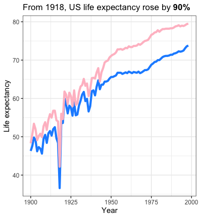
Finally, we can visualize the changes in life expectancy across the $20^{th}$ century. From a low point in 1918, life expectancy rose 1.9-fold.
us_life_expectancy_tbl %>%
  tidyr::gather(sex, life_expectancy, -Year) %>%
  mutate(sex = factor(sex, levels = c("M", "F"))) %>%
  ggplot(aes(x = Year, y = life_expectancy, color = sex)) +
  geom_path(linewidth = 2) +
  scale_y_continuous("Life expectancy") +
  scale_x_continuous("Year") +
  scale_color_manual(
    values = c("F" = "pink", "M" = "dodgerblue")
  ) +
  labs(title = "From 1918, US life expectancy rose by **90%**"
  ) +
  theme_bw_mod +
  theme(
    legend.position = "none",
    plot.title = ggtext::element_markdown(size = 17, lineheight = 1.2)
  )
Unpacking the Gompertz Equation
As mentioned above, the form of the Gompertz equation is:
\[\large \ln(h(t)) = \ln(\alpha) + \beta \cdot t \\ \large h(t) = \alpha \cdot e^{\beta \cdot t}\]For a given, value of $\alpha$ and $\beta$ we could use the Gompertz equation to predict an individual’s hazard at an age $t$.
Surviving to an age $t$ entails surviving every preceding year as well. Thus, the survival function can be described as the probability of surviving until a point $t$:
\[\large S(t) = \prod_{x=1}^{t}\left(1-h(x)\right)\]For the survival function, this is analytically equivalent to:
\[\large S(t) = e^{\frac{\alpha}{\beta}(1-e^{\beta t})}\]Also, since life expectancy is defined “assuming that the age-specific death rates for the year in question will apply throughout the lifetime of individuals born in that year” it should simply be the integral under the survival curve (or the sum since we are discretizing to year-by-year changes).
Based on this formulation I wrote equations which map $\alpha$, $\beta$ and $t$ onto hazard and survival and created plots which summarize a Gompertz model approximately fitting to the modern US population.
gompertz_hazard <- function(alpha, beta, times) {
  alpha*exp(beta*times)
}

gompertz_survival <- function(alpha, beta, times) {
  exp((alpha/beta)*(1-exp(beta*times)))
}

# doubling of hazard every 8 years
BETA_CURRENT = 0.0861
ALPHA_CURRENT = 0.000064
AGES <- seq(1, 105)

#
gompertz_df <- tibble::tibble(
  age = AGES,
  hazard = gompertz_hazard(ALPHA_CURRENT, BETA_CURRENT, AGES)
) %>%
  mutate(
    log_hazard = log(hazard),
    survival = gompertz_survival(ALPHA_CURRENT, BETA_CURRENT, AGES)
    )

# the integral of survival is life expectancy
life_expectancy <- sum(gompertz_df$survival)

hazard_grob <- ggplot(gompertz_df, aes(x = age, y = hazard)) +
  geom_point() +
  theme_bw_mod

survival_grob <- ggplot(gompertz_df, aes(x = age, y = survival)) +
  geom_polygon(
    data = dplyr::bind_rows(
      gompertz_df,
      tibble::tibble(age = 0, survival = 0),
      tibble::tibble(age = 0, survival = 1)
      ),
    fill = "blue", alpha = 0.2) +
  geom_point() +
  geom_vline(xintercept = life_expectancy, color = "blue", width = 2) +
  annotate("text", x = life_expectancy - 2, y = 0.25, label = "life expectancy", color = "blue", hjust = 1) +
  theme_bw_mod
## Warning in geom_vline(xintercept = life_expectancy, color = "blue", width = 2):
## Ignoring unknown parameters: `width`log_hazard_grob <- ggplot(gompertz_df, aes(x = age, y = log_hazard)) +
geom_point() +
scale_y_continuous("log(hazard)") +
theme_bw_mod
log_hazard_grob + hazard_grob + survival_grob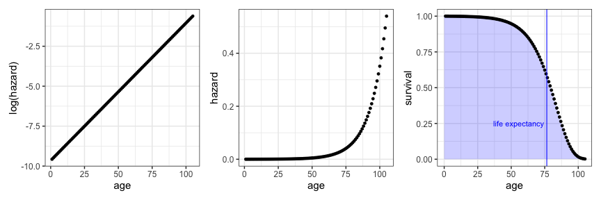
To do this, I fixed $\beta$ at the value of 0.0861 which imputes a doubling of risk every 8 years. Since it is widely believed that historical lifespan extension has primarily been through modifying $\alpha$ rather than $\beta$ we can fit Gompertz models to achieve a desired life expectancy. For a life expectancy of around 76.6 (the life expectancy in 1998 which is also startling close to the current life expectancy in the USA of 77.2), $\alpha$ would be $\sim0.000064$.
To explore how $\alpha$ has changed across the $20^{th}$ century we can explore how different levels of baseline risk map onto historical changes in life expectancy.
20th century lifespan extension was through a 26x drop in baseline hazard
To map values of $\alpha$ onto the “select_lifespans” defined above, I estimated the Gompertz survival function for a range of $\alpha$ values starting at a modern value of $\sim0.000064$ and going down to a 26-fold decrease in $\alpha$ (initially I did a wider range then I dialed it in). Tidyr’s crossing is really helpful for doing the all-by-all comparisons of the set of $\alpha$ parameters and ages being evaluated. After calculating the survival functions I grouped by $\alpha$ parameters and integrated over ages to infer the life expectancy.
# define fold-change of max/min alpha or beta
ALPHA_BETA_FC = 26

# create a uniform sequence in log-space (the log transform is just so ages will be evenly space when plotting lifespan ~ log(param)
alpha_possibilities = exp(seq(log(ALPHA_CURRENT), log(ALPHA_CURRENT*ALPHA_BETA_FC), length.out = 100))

gompertz_curves <- tidyr::crossing(alpha = alpha_possibilities, age = AGES) %>%
  mutate(survival = gompertz_survival(alpha, BETA_CURRENT, age))

life_expectancy_by_alpha <- gompertz_curves %>%
  summarize(life_expectancy = sum(survival), .by = alpha)

# what is the alpha corresponding to the selected years life expectancies
select_lifespans_w_alpha <- select_lifespans %>%
  tidyr::crossing(life_expectancy_by_alpha) %>%
  mutate(year_lifespan_vs_alpha_prediction = abs(avg_lifespan - life_expectancy)) %>%
  group_by(Year) %>%
  filter(year_lifespan_vs_alpha_prediction == min(year_lifespan_vs_alpha_prediction))

stopifnot(all(select_lifespans_w_alpha$year_lifespan_vs_alpha_prediction < 1))

life_expectancy_by_alpha %>%
  ggplot(aes(x =  log10(alpha), y = life_expectancy)) +
  geom_point() +
  ggrepel::geom_text_repel(data = select_lifespans_w_alpha, aes(x = log10(alpha), y = life_expectancy, label = Year), force = 50, hjust = 0, nudge_x = 0.06, nudge_y = 1.5) +
  scale_x_continuous(expression(log[10] ~ alpha)) +
  scale_y_continuous("Life expectancy") +
  labs(title = "20<sup>th</sup> century lifespan extension was primarily <br>through a **26x** drop in baseline hazard") +
  theme_bw_mod +
  theme(
    plot.title = ggtext::element_markdown(size = 13, lineheight = 1.2)
  )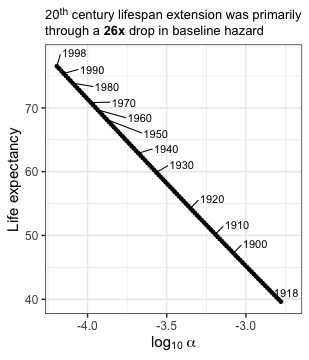
The nearly doubling of life expectancy across the $20^{th}$ century was chiefly driven by the massive medical advancements of antibiotics and vaccines, as well improvements in nutrition and hygiene. The deceleration of lifespan extension over the last thirty years reflects the challenge of removing risks one-by-one like in a game of wack-a-mole. Going forward, little is projected to change as judged by the social security administration, where lifespan extension in 2,100 is only projected to reach $\sim85$ years
These are and will-be, hard fought for gains, but radically extending lifespan should tackle the underlying risk factors of diseases of aging … aging itself.
A 26x drop in age-dependent risk would increase human life expectancy by 12.5x
The 26-fold drop in age-independent hazard across the 20th century is MASSIVE and I was curious what a comparable drop in $\beta$ going forward would look like. To explore this, I fixed $\alpha$ at a modern value (0.000064) and explored a range of $\beta$ values ranging from the current value (0.0861; where risk would double every 8 years) down to 0.0033 where risk would double every 208 years.
AGES_EXTENDED <- seq(0, 100000)
beta_possibilites = exp(seq(log(BETA_CURRENT), log(BETA_CURRENT/ALPHA_BETA_FC), length.out = 100))

gompertz_curves <- tidyr::crossing(beta = beta_possibilites, age = AGES_EXTENDED) %>%
  mutate(
    hazard = gompertz_hazard(ALPHA_CURRENT, beta, age),
    survival = gompertz_survival(ALPHA_CURRENT, beta, age)
  )

life_expectancy_by_beta <- gompertz_curves %>%
  summarize(life_expectancy = sum(survival), .by = beta)

life_expectancy_range_ratio <- life_expectancy_by_beta$life_expectancy[1] / life_expectancy_by_beta$life_expectancy[nrow(life_expectancy_by_beta)]

life_expectancy_by_beta %>%
  ggplot(aes(x = log10(beta), y = life_expectancy)) +
  geom_point() +
  scale_x_continuous(expression(log[10] ~ beta), breaks = seq(-5, 1, by = 0.5), expand = c(0.02,0.02)) +
  scale_y_continuous("Life expectancy") +
  labs(title = "A **26x** drop in age-dependent risk would<br>increase human lifespan by **12.5x**") +
  theme_bw_mod +
  theme(
    plot.title = ggtext::element_markdown(size = 14, lineheight = 1.2)
  )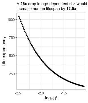
I don’t think it will be as easy to modify $\beta$ as $\alpha$ even a two-fold drop in $\beta$ would increase life expectancy to 138 years. Precipitously dropping $\beta$ and achieving a life expectancy of 1,000 is starting to sound like science fiction but it is an interesting thought experiment. But why stop there! We can push this further and explore what a world with a $\beta$ of zero would look like. This concept is reflected in an interesting game by Polstats where you can simulate 100 individual’s lifespans in a world where you only die of unnatural causes. The average lifespan in this cohort was ~10,000 years old and the longest lived individual died at the ripe old age of 57,912 in a car accident.
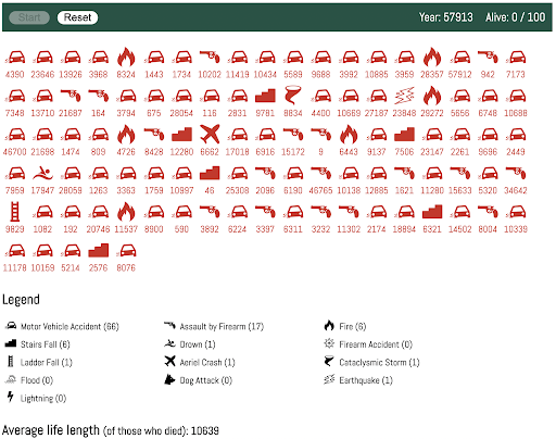
Playing this game a few times I was struck by how much the average lifespan of the cohort can shift based on a few long-lived stragglers who continue to dodge bullets (and cars).
In this world, how old would we expect the oldest person to be?
If hazard is constant over time then lifespans would follow a Geometric distribution, where the mean equals (1/$\alpha$ = 15,625). If we thought of lifespans as continuous in nature, which would be appropriate, then we could similarly think of lifespans as following an exponential distribution (equivalent to exponential decay).
tibble(age = seq(0, 100000, by = 50)) %>%
  mutate(survival = dgeom(age, ALPHA_CURRENT)) %>%
  ggplot(aes(x = age, y = survival)) +
  geom_path() +
  theme_bw_mod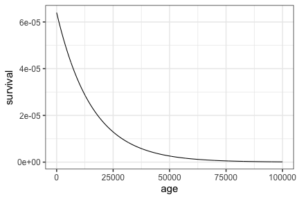
The maximum lifespan under this model would be equivalent to the maximum of $N$ geometric draws. This distribution is described in StackExchange and its quite involved (there’s no cgeom function), so I’ll cop out and just obtain the maximum value of a set of random draws.
set.seed(1234)
current_earth_pop_w_geometric_lifespan <- rgeom(n = 7.9e9, ALPHA_CURRENT)
max_lifespan <- max(current_earth_pop_w_geometric_lifespan)
From this simulation the maximum age of the oldest person on earth would be 345,353 years old.
Conclusion
In this post, we’ve explored the Gompertz equation and how it can be used to model historical lifespan extention (decreasing $\alpha$) and the potential that slowing aging has for radical lifespan extension (decreasing $\beta$).
I’ve found that this framing is particularly helpful when discussing my professional work with non-scientists. I tried this out first in a presentation at a local meetup (Future Tech Immersive: AI x Synthetic Biology Meetup) and simplified the narrative last November when I spoke at the 2024 D One Growing Together Conference in Zürich. Both talks went quite well - aging is deeply personal to all of us. Its something we see every day in ourselves, our family, and our friends. We accept it as a given, but it may not be and that “what if?” continues to inspire me.
Leave a comment