Network Biology with Napistu, Part 1: Creating Multimodal Disease Profiles

This is part one of a two-part post highlighting Napistu — a new framework for building genome-scale networks of molecular biology and biochemistry. In this post, I’ll tackle a fundamental challenge in computational biology: how to extract meaningful disease signatures from complex multimodal datasets.

Using methylmalonic acidemia (MMA) as my test case, I’ll demonstrate how to systematically extract disease signatures from multimodal data. My approach combines three complementary analytical strategies: exploratory data analysis to assess data structure and quality, differential expression analysis to identify disease-associated features, and factor analysis to uncover coordinated gene expression programs across data types. The end goal is to distill thousands of molecular measurements into a handful of interpretable disease signatures — each capturing a distinct aspect of disease biology that can be mapped to regulatory networks.

Throughout this post, I’ll use two types of asides to provide additional context without disrupting the main analytical flow. Green boxes contain biological details, while blue boxes reflect on the computational workflow and AI-assisted development process.

For biologists: I identify a previously unreported batch effect related to sample freezing dates that impacts both data modalities. By accounting for this and other technical covariates, I demonstrate improved power to detect disease-relevant associations in the proteomics dataset. I also show that urine MMA levels exhibit stronger statistical associations with molecular features than traditional enzyme activity measures in this dataset. In part two, I will link these statistical associations to upstream regulators using a genome-scale mechanistic network, enabling me to define a regulon underlying the molecular pathophysiology of MMA.

For computational folks: While developing this analysis and the underlying software, I intentionally explored AI-assisted coding across the full development lifecycle — from building statistical pipelines in Python to contributing to Napistu, a complex scientific programming framework for network biology. I’ll share specific examples where AI excelled (e.g., rapid prototyping, API exploration) and where it failed in potentially dangerous ways (e.g., confusing p-values with q-values, breaking regression formulas). I’ll also offer practical strategies for maintaining code quality while working at AI speed.

What is Methylmalonic acidemia?

Methylmalonic acidemia (MMA) — not to be confused with mixed martial arts (which I used to blog about at Fight Prior) — is an inborn error of metabolism characterized by the buildup of methylmalonic acid.

MMA is genetically heterogeneous, caused by defects in approximately 20 genes involved in propionate metabolism. Classical isolated MMA is primarily due to autosomal recessive mutations in the enzyme methylmalonyl-CoA mutase (MMUT), which converts methylmalonyl-CoA to succinyl-CoA as part of the propionate catabolic pathway. This pathway processes metabolites derived from odd-chain fatty acids, cholesterol, and certain amino acids. When disrupted, methylmalonic acid accumulates, leading to metabolic acidosis and multi-organ dysfunction, including neurological abnormalities, kidney failure, and growth impairment.

Despite being linked to a well-characterized metabolic pathway, MMA presents significant clinical and research challenges. Patients exhibit substantial variability in disease severity, treatment responsiveness, and clinical outcomes—even among those with identical genetic mutations. While traditional biochemical assays provide valuable diagnostic information, they offer only a partial view of disease pathophysiology. This variability suggests that understanding MMA requires moving beyond simple “broken enzyme” models toward systems-level approaches capable of capturing the complex downstream effects of metabolic disruption.

The Forny multi-omics approach

To address the complexity of MMA, Forny et al., 2023 conducted one of the largest multi-omics studies of a rare metabolic disorder. They profiled 210 patient-derived fibroblast lines and 20 controls using transcriptomics and proteomics to better understand disease etiology and identify potential therapeutic interventions.

The study achieved a molecular diagnosis in 177 out of 210 cases (84%), though 33 patients remained without a clear genetic explanation. While 148 patients had MMUT mutations, others carried defects in ACSF3, TCN2, SUCLA2, and additional genes — revealing broader genetic heterogeneity than previously recognized. Beyond diagnostic insights, the study uncovered unexpected disruption of TCA cycle anaplerosis (metabolic replenishment pathways), particularly involving glutamine metabolism. It also identified physical interactions between MMUT and other metabolic enzymes, suggesting coordinated regulation, and demonstrated that dimethyl-oxoglutarate treatment can restore metabolic function in cellular models.

The findings suggest that MMA involves more than just a “broken enzyme.” MMUT deficiency triggers a systematic rewiring of cellular metabolism, especially in how cells replenish TCA cycle intermediates. This anaplerotic shift includes increased reliance on glutamine metabolism and appears to involve direct protein-protein interactions between MMUT and glutamine-processing enzymes. These results indicate that MMUT may function as part of a larger metabolic regulatory complex — an unexpected insight with potential therapeutic implications.

While the Forny study made significant advances, it also highlighted a fundamental puzzle. MMA exhibits many features of a classical autosomal recessive metabolic disorder: patients have well-defined enzymatic defects, and some respond to metabolic interventions, such as vitamin supplementation. Yet, the presence of treatment-resistant cases, highly variable disease severity, and patients without clear genetic explanations suggest that MMA pathophysiology extends beyond mere metabolic dysfunction.

This paradox suggests that MMA may be influenced by broader regulatory networks that either shape cellular metabolism or respond dynamically to its disruption. If this is the case, understanding MMA requires moving beyond metabolic modeling and adopting approaches that simultaneously capture both metabolic and genic regulatory mechanisms. To address this challenge, I aim to create molecular disease signatures that can be mapped onto biological networks linking metabolic pathways to their upstream regulatory controls. Rather than viewing MMA solely as a metabolic disorder, this systems-level approach treats gene-centric and metabolism-centric regulation as interconnected, enabling me to trace disease signals from downstream molecular effects to potential upstream drivers.

Strategy for creating disease profiles

To create interpretable disease signatures from the Forny dataset, I’ll follow a systematic approach:

1. Preprocessing: Address missing phenotype data and technical covariates
2. Exploratory analysis: Identify batch effects and major sources of variation
3. Supervised regression: Find individual disease-associated features
4. Unsupervised factor analysis: Discover coordinated multi-omic programs

AI as a development collaborator

While I typically perform exploratory data analysis and statistical analysis in R, I implemented this analysis in Python. This provided an opportunity to explore AI-assisted development — not as a replacement for careful software engineering, but as a collaborator for writing and testing code more efficiently. Throughout the analysis, I’ll highlight specific examples of where this approach succeeded and where it fell short.

Creating molecular profiles of MMA

Environment setup

If you’d like to reproduce this analysis, follow these steps:

1. Install uv (or just use pip install)

2. Setup a Python environment:

   uv venv --python 3.11
   source .venv/bin/activate
   
   # Core dependencies
   uv pip install napistu'[scverse]'
   # Personal utilities package with genomics analysis functions
   uv pip install "git+https://github.com/shackett/shackett-utils.git[all]" 
   # Additional dependencies
   uv pip install openpyxl scikit-learn mofapy2 ipykernel
   python -m ipykernel install --user --name=forny-2023
   

3. Download Source Data Fig.1 and Source Data Fig.2 from Forny et al., 2023

4. Set the paths in the following code block:

   a. SUPPLEMENTAL_DATA_DIR should point to the directory containing the download from step 3 (“42255_2022_720_MOESM3_ESM.xlsx” and “42255_2022_720_MOESM4_ESM.xlsx”) b. CACHE_DIR should point to a location where intermediate results and outputs can be saved

5. Run the notebook and render an html output:

   quarto render creating_multimodal_profiles.qmd
   

First, I’ll load the necessary Python modules, configure paths, set global parameters, and define utility functions.

import os
import textwrap

import anndata as ad
import matplotlib.pyplot as plt
import mudata as md
import muon
import numpy as np
import pandas as pd
import scanpy as sc
import seaborn as sns
from sklearn.impute import KNNImputer
from IPython.display import display, HTML

# this analysis is largely upstream of Napistu but we can use some of its utils
from napistu import utils as napistu_utils

# import local modules
from shackett_utils.applications import forny_imputation
import shackett_utils.genomics.adata_processing as processing
from shackett_utils.genomics import adata_regression
from shackett_utils.genomics import mdata_eda
from shackett_utils.genomics import mdata_factor_analysis
from shackett_utils.statistics import stats_viz
from shackett_utils.statistics import transform

# File paths and data organization
# All input data should be placed in the SUPPLEMENTAL_DATA_DIR
# Cached results and models will be stored in CACHE_DIR

# paths
PROJECT_DIR = os.path.expanduser("~/napistu_mma_posts")
SUPPLEMENTAL_DATA_DIR = os.path.join(PROJECT_DIR, "input")
CACHE_DIR = os.path.join(PROJECT_DIR, "cache")

# Define the path to save hyperparameter scan results
MOFA_PARAM_SCAN_MODELS_PATH = os.path.join(CACHE_DIR, "mofa_param_scan_h5mu")
# Final results 
OPTIMAL_MODEL_H5MU_PATH = os.path.join(CACHE_DIR, "mofa_optimal_model.h5mu")

# formats
SUPPLEMENTAL_DATA_FILES = {
    "transcriptomics" : {
        "file" : "42255_2022_720_MOESM3_ESM.xlsx",
        "sheet" : "Source Data transcriptomics"
    },
    "proteomics" : {
        "file" : "42255_2022_720_MOESM3_ESM.xlsx",
        "sheet" : "Source Data proteomics"
    },
    "phenotypes" : {
        "file" : "42255_2022_720_MOESM4_ESM.xlsx",
        "sheet" : 0
    }
}

# other globals
# path to proteomics filenames for extracting run order
PROTEOMICS_FILE_NAMES_URL = "https://github.com/user-attachments/files/20616164/202502_PHRT-5_MMA_Sample-annotation.txt"
# filter genes with fewer than this # of counts summed over samples
READ_CUTOFF = int(400)
# filter phenotypes with more than this # of missing values
MAX_MISSING_PHENOTYPE = int(180)
# measure to use for analysis
ANALYSIS_LAYER = "log2_centered"
# cutoff for qvalues (FDR-adjusted p-values)
FDR_CUTOFF = 0.1
# Overwrite the results if they already exist   
OVERWRITE = False
# Define the optimal number of factors
OPTIMAL_FACTOR = int(30)
# Define the range of factors to test for MOFA
FACTOR_RANGE = range(4, 51, 2)
# naming scheme for feature- and factor-level regression results
FEATURE_REGRESSION_STR = "feature_regression_{}"
FACTOR_REGRESSION_STR = "mofa_regression_{}"

# Statistical model specifications
# Used for both feature- and factor-level regression
# We use different covariates for each data modality based on identified batch effects:
# - Transcriptomics: only date_freezing affects expression
# - Proteomics: both proteomics_runorder and date_freezing are significant
# The 's()' notation indicates spline smoothing for non-linear relationships
REGRESSION_FORMULAS = {
    "transcriptomics" : {
        "case" : "~ case + s(date_freezing)",
        "OHCblPlus" : "~ OHCblPlus + s(date_freezing)",
        "MMA_urine" : "~ MMA_urine + s(date_freezing)",
        "responsive_to_acute_treatment" : "~ responsive_to_acute_treatment + s(date_freezing)",
        "proteomics_runorder" : "~ s(proteomics_runorder) + s(date_freezing)", # we don't expect this to be significant
        "date_freezing" : "~ s(proteomics_runorder) + s(date_freezing)"
    },
    "proteomics" : {
        "case" : "~ case + s(proteomics_runorder) + s(date_freezing)",
        "OHCblPlus" : "~ OHCblPlus + s(proteomics_runorder) + s(date_freezing)",
        "MMA_urine" : "~ MMA_urine + s(proteomics_runorder) + s(date_freezing)",
        "responsive_to_acute_treatment" : "~ responsive_to_acute_treatment + s(proteomics_runorder) + s(date_freezing)",
        "proteomics_runorder" : "~ s(proteomics_runorder) + s(date_freezing)",
        "date_freezing" : "~ s(proteomics_runorder) + s(date_freezing)"
    }
}

# utility functions

def create_stacked_barplot_from_regression(regression_results_df, q_threshold=FDR_CUTOFF):
    """
    Create a stacked barplot showing significant results by modality and model_name
    
    Parameters:
    regression_results_df: DataFrame with columns including 'q_value', 'modality', 'model_name'
    q_threshold: significance threshold for q_value (default: 0.1)
    """
    # Get significant results using your counting logic
    significant_counts = regression_results_df.query(f"q_value < {q_threshold}").value_counts(["modality", "model_name"])
    
    # Convert to DataFrame for easier manipulation
    df = significant_counts.reset_index()
    df.columns = ['modality', 'model_name', 'count']
    
    # Get all unique model_names from the original dataframe to ensure they all appear
    all_model_names = regression_results_df['model_name'].unique()
    all_modalities = regression_results_df['modality'].unique()
    
    # Create a complete DataFrame with all combinations, filling missing with 0
    from itertools import product
    all_combinations = pd.DataFrame(
        list(product(all_modalities, all_model_names)), 
        columns=['modality', 'model_name']
    )
    all_combinations['count'] = 0
    
    # Merge with actual counts, keeping all combinations
    df_complete = all_combinations.merge(
        df, on=['modality', 'model_name'], 
        how='left', suffixes=('_empty', '_actual')
    )
    
    # Use actual counts where available, otherwise use 0
    df_complete['count'] = df_complete['count_actual'].fillna(df_complete['count_empty'])
    df_complete = df_complete[['modality', 'model_name', 'count']]
    
    # Set seaborn style
    sns.set_style("whitegrid")
    
    # Group by model_name and sum counts across modalities to get total counts for ordering
    total_counts = df_complete.groupby('model_name')['count'].sum().sort_values(ascending=False)
    
    # Create pivot table with model_name as index and modality as columns
    pivot_df = df_complete.pivot_table(index='model_name', columns='modality', values='count', fill_value=0)
    
    # Reorder by total counts (descending)
    pivot_df = pivot_df.reindex(total_counts.index)
    
    # Create the plot
    fig, ax = plt.subplots(figsize=(14, 8))
    
    # Use seaborn color palette
    colors = sns.color_palette("husl", len(pivot_df.columns))
    
    # Plot stacked bars
    pivot_df.plot(kind='bar', stacked=True, ax=ax, color=colors, alpha=0.8)
    
    # Customize the plot
    ax.set_title(f'Significant Results by Model Name and Modality (q < {q_threshold})', fontsize=16, fontweight='bold')
    ax.set_xlabel('Model Name (ordered by total significant count)', fontsize=12)
    ax.set_ylabel('Count of Significant Results', fontsize=12)
    ax.legend(title='Modality', bbox_to_anchor=(1.05, 1), loc='upper left')
    
    # Add total count labels at the top of each bar
    for i, (model_name, total_count) in enumerate(total_counts.items()):
        if total_count > 0:  # Only show label if there are any significant results
            ax.text(i, total_count + max(total_counts) * 0.01, str(int(total_count)), 
            ha='center', va='bottom', fontweight='bold', fontsize=10)
    
    # Rotate x-axis labels for better readability
    plt.xticks(rotation=45, ha='right')
    plt.tight_layout()
    
    plt.show()
    
    return fig, ax, pivot_df

def runorder_from_filename(fn: str) -> int:
    """Retrieve runorder form filename

    Args:
        fn (str): Filename ending in runorder

    Returns:
        runorder
    Example:
        >>> runorder_from_filename("asdf_2")
        2
    """
    return int(fn.split("_")[-1])

# load data
supplemental_data_path = {
    x : {
        "path" : os.path.join(SUPPLEMENTAL_DATA_DIR, y["file"]),
        "sheet" : y["sheet"]
    }
        for x, y in SUPPLEMENTAL_DATA_FILES.items()
}

assert all([os.path.isfile(x["path"]) for x in supplemental_data_path.values()])

Next, I’ll load the transcriptomics and proteomics datasets (stored in separate sheets of the same Excel file), along with the phenotypic data.

supplemental_data = {
    x : pd.read_excel(y["path"], sheet_name = y["sheet"]) for x, y in supplemental_data_path.items()
}

# formatting
supplemental_data["transcriptomics"] = (
    supplemental_data["transcriptomics"]
    .rename({"Unnamed: 0" : "ensembl_gene"}, axis = 1)
    .set_index("ensembl_gene")
)
supplemental_data["proteomics"] = (
    supplemental_data["proteomics"]
    .rename({"PG.ProteinAccessions" : "uniprot"}, axis = 1)
    .set_index("uniprot")
)
supplemental_data["phenotypes"] = (
    supplemental_data["phenotypes"]
    .rename({"Unnamed: 0" : "patient_id"}, axis = 1)
    .set_index("patient_id")
)

Data overview

The Forny et al. dataset contains three key components:

• Transcriptomics: RNA-seq data from patient-derived fibroblasts (210 MMA patients + 20 controls)
• Proteomics: Mass spectrometry data from the same cell lines
• Phenotypes: Clinical measurements including enzymatic assays and biochemical markers. The main disease phenotypes I will focus on are:
  • case: A binary variable indicating whether individuals exhibit clinical MMA or are healthy controls
  • responsive_to_acute_treatment: A binary variable indicating whether patients show clinical improvement following acute vitamin supplementation interventions
  • OHCblPlus: A quantitative measure of methylmalonyl-CoA mutase enzyme activity, where higher values indicate better enzymatic function
  • MMA_urine: A quantitative measurement of methylmalonic acid levels in urine, where elevated levels indicate metabolic dysfunction and greater disease severity

Key analytical challenges include severe class imbalance (only 20 controls versus 210 cases), missing phenotype data for many clinical measurements, potential technical variation from sample processing, and disease heterogeneity, characterized by varying genetic subtypes and levels of severity.

Formatting phenotypes and technical covariates

Clinical data present unique challenges that require careful preprocessing. Measurements are often right-skewed and contain missing values because only a subset of tests is typically ordered for each patient. Since I’m interested in quantitative biomarkers, having complete data across patients increases statistical power. While imputation can address missingness, it is beneficial to first transform the variables to more closely approximate a multivariate Gaussian distribution. This transformation also enhances regression modeling by linearizing relationships between dependent and independent variables.

A critical aspect of this dataset is accounting for technical variation. The proteomics data were collected across different instrument runs, and I can extract the run order from the original PRIDE repository filenames. This run order represents a major source of variation that must be controlled in my statistical models.

# load run order
proteomics_file_names = pd.read_csv(PROTEOMICS_FILE_NAMES_URL, sep = "\t")
proteomics_file_names["proteomics_runorder"] = [runorder_from_filename(fn) for fn in proteomics_file_names["File Name"]]
proteomics_file_names["patient_id"] = proteomics_file_names["Run Label"].str.replace("_", "")
# some samples have multiple files in the PRIDE proteomics repository but they each sample is just a single observation in the
# final dataset. Here we'll take the max run order for each patient. These likely reflect reruns due to technical failures
# so the max run order sample is usually the one with the best technical quality.
proteomics_file_names = proteomics_file_names.groupby("patient_id")["proteomics_runorder"].max()

# select continuos phenotypes without too many missing values
continuous_df = forny_imputation._select_continuous_measures(supplemental_data["phenotypes"], max_missing = MAX_MISSING_PHENOTYPE)

# identify transformations which improve variable normality
normalizing_transforms = {}
for col in continuous_df.columns:
    normalizing_transforms[col] = transform.best_normalizing_transform(continuous_df[col])["best"]
    
func_transform_dict = {col: transform.transform_func_map[trans] for col, trans in normalizing_transforms.items()}

# Apply transformation
transformed_df = forny_imputation.transform_columns(continuous_df, func_transform_dict)

# Create the imputer
imputer = KNNImputer(n_neighbors=5, weights="uniform")

# Fit and transform the data
imputed_array = imputer.fit_transform(transformed_df)
imputed_df = pd.DataFrame(imputed_array, columns=transformed_df.columns, index=transformed_df.index)

binary_phenotypes = supplemental_data["phenotypes"][[col for col in supplemental_data["phenotypes"].columns if supplemental_data["phenotypes"][col].dropna().nunique() == 2]]

# create a table of phenotypes
phenotypes_df = (
    pd.concat([
        binary_phenotypes,
        imputed_df
    ], axis = 1)
    # add proteomics run order since this is a batch effect in the proteomics data
    .join(proteomics_file_names, how = "left")
)

forny_imputation.plot_clustered_correlation_heatmap(transformed_df)

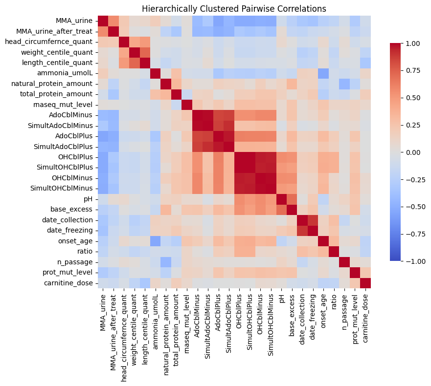
The correlation heatmap reveals important structure within the clinical data. Block-diagonal patterns show related assays clustering together: AdoCbl assays correlate strongly with one another, OHCbl assays form a distinct cluster, and both are anti-correlated with MMA excretion into urine. This correlation structure supports my use of a K-Nearest Neighbors imputation strategy.

To create the transformation module for identifying optimal normalizing transformations, I began by providing high-level problem guidance to Claude. Initially, it produced overly complicated code focused on finding transformations that would yield Kolmogorov–Smirnov (KS) test p-values greater than 0.05 for assessing normality. While it suggested useful transformations like Box-Cox and Yeo-Johnson, it also recommended quantile normalization — which, although effective at making data Gaussian, defeats the purpose of preserving the original data’s distribution. The criterion of accepting only transformations with p > 0.05 was problematic, since KS tests are almost always significant when comparing real-world data to parametric distributions. With further guidance and iterative refinement in Cursor, the final module performed well. Claude was especially helpful in handling matplotlib’s tricky syntax, enabling me to quickly create complex, specialized plots for visualizing missing value patterns and comparing transformations.

Organizing results with scverse

To make my analysis more reproducible and compatible with the broader genomics ecosystem, I’ll organize my data using the scverse framework. This ecosystem, built around AnnData and MuData objects, provides standardized containers for genomics data that integrate observation metadata, feature annotations, and multiple data layers.

Using AnnData/MuData offers several advantages:

• Standardization: A common format across the Python genomics ecosystem
• Integration: Easy to combine with existing tools like scanpy, muon, and scvi-tools
• Metadata management: Keeps sample annotations and results together
• Multimodal support: Native integration of any combination of data modalities

transcr_adata = ad.AnnData(
    X = supplemental_data["transcriptomics"].T,
    # some samples are missing
    obs = phenotypes_df.loc[phenotypes_df.index.isin(supplemental_data["transcriptomics"].columns)],
)

protein_metadata_vars = supplemental_data["proteomics"].columns[supplemental_data["proteomics"].columns.str.startswith("PG")]

proteomics_adata = ad.AnnData(
    # drop protein metadata vars and transpose
    X = supplemental_data["proteomics"].drop(protein_metadata_vars, axis = 1).T,
    # some samples are missing
    obs = phenotypes_df.loc[phenotypes_df.index.isin(supplemental_data["proteomics"].columns)],
    var = supplemental_data["proteomics"][protein_metadata_vars],
)

mdata = md.MuData({"transcriptomics": transcr_adata, "proteomics": proteomics_adata})
mdata

MuData object with n_obs × n_vars = 230 × 19537
  2 modalities
    transcriptomics:    221 x 14749
      obs:  'case', 'gender', 'consanguinity', 'mut_category', 'wgs_zygosity', 'acidosis', 'metabolic_acidosis', 'metabolic_ketoacidosis', 'ketosis', 'hyperammonemia', 'abnormal_muscle_tone', 'musc_hypotonia', 'musc_hypertonia', 'fct_respiratory_abnormality', 'dyspnea', 'tachypnea', 'reduced_consciousness', 'lethargy', 'coma', 'seizures', 'general_tonic_clonic_seizure', 'any_GI_problem', 'failure_to_thrive', 'any_delay', 'behavioral_abnormality', 'concurrent_infection', 'urine_ketones', 'dialysis', 'peritoneal_dialysis', 'insulin', 'diet', 'carnitine', 'cobalamin', 'bicarb', 'glucose_IV', 'cobalamin_responsive', 'antibiotic_treatment', 'protein_restriction', 'tube_feeding_day', 'tube_feeding_night', 'tube_feeding_overall', 'language_delay', 'any_neurological_abnormalities_chronic', 'impaired_kidney_fct', 'hemat_abnormality', 'anemia', 'neutropenia', 'skin_abnormalities', 'hearing_impairment', 'osteoporosis', 'failure_to_thrive_chronic', 'global_dev_delay_chr', 'hypotonia_chr', 'basal_ganglia_abnormality_chr', 'failure_to_thrive_or_tube_feeding', 'irritability', 'hyperventilation', 'hypothermia', 'somnolence', 'vomiting', 'dehydration', 'feeding_problem', 'responsive_to_acute_treatment', 'n_passage', 'date_collection', 'date_freezing', 'onset_age', 'OHCblMinus', 'OHCblPlus', 'ratio', 'SimultOHCblMinus', 'SimultOHCblPlus', 'AdoCblMinus', 'AdoCblPlus', 'SimultAdoCblMinus', 'SimultAdoCblPlus', 'prot_mut_level', 'rnaseq_mut_level', 'MMA_urine', 'ammonia_umolL', 'pH', 'base_excess', 'MMA_urine_after_treat', 'carnitine_dose', 'natural_protein_amount', 'total_protein_amount', 'weight_centile_quant', 'length_centile_quant', 'head_circumfernce_quant', 'proteomics_runorder'
    proteomics: 230 x 4788
      obs:  'case', 'gender', 'consanguinity', 'mut_category', 'wgs_zygosity', 'acidosis', 'metabolic_acidosis', 'metabolic_ketoacidosis', 'ketosis', 'hyperammonemia', 'abnormal_muscle_tone', 'musc_hypotonia', 'musc_hypertonia', 'fct_respiratory_abnormality', 'dyspnea', 'tachypnea', 'reduced_consciousness', 'lethargy', 'coma', 'seizures', 'general_tonic_clonic_seizure', 'any_GI_problem', 'failure_to_thrive', 'any_delay', 'behavioral_abnormality', 'concurrent_infection', 'urine_ketones', 'dialysis', 'peritoneal_dialysis', 'insulin', 'diet', 'carnitine', 'cobalamin', 'bicarb', 'glucose_IV', 'cobalamin_responsive', 'antibiotic_treatment', 'protein_restriction', 'tube_feeding_day', 'tube_feeding_night', 'tube_feeding_overall', 'language_delay', 'any_neurological_abnormalities_chronic', 'impaired_kidney_fct', 'hemat_abnormality', 'anemia', 'neutropenia', 'skin_abnormalities', 'hearing_impairment', 'osteoporosis', 'failure_to_thrive_chronic', 'global_dev_delay_chr', 'hypotonia_chr', 'basal_ganglia_abnormality_chr', 'failure_to_thrive_or_tube_feeding', 'irritability', 'hyperventilation', 'hypothermia', 'somnolence', 'vomiting', 'dehydration', 'feeding_problem', 'responsive_to_acute_treatment', 'n_passage', 'date_collection', 'date_freezing', 'onset_age', 'OHCblMinus', 'OHCblPlus', 'ratio', 'SimultOHCblMinus', 'SimultOHCblPlus', 'AdoCblMinus', 'AdoCblPlus', 'SimultAdoCblMinus', 'SimultAdoCblPlus', 'prot_mut_level', 'rnaseq_mut_level', 'MMA_urine', 'ammonia_umolL', 'pH', 'base_excess', 'MMA_urine_after_treat', 'carnitine_dose', 'natural_protein_amount', 'total_protein_amount', 'weight_centile_quant', 'length_centile_quant', 'head_circumfernce_quant', 'proteomics_runorder'
      var:  'PG.ProteinDescriptions', 'PG.ProteinNames', 'PG.Qvalue'

Data normalization

Following the methodology from Forny et al., I will apply a three-step normalization process designed to make the data more suitable for statistical analysis:

1. Filtering poorly measured features: Remove genes with very few reads across samples
2. Log-transformation: Stabilize variance and make distributions more Gaussian (necessary because I’m working with processed data rather than original counts)
3. Row and column centering: Remove systematic biases like library size effects while preserving biological signal (following the Forny methodology)

# filter to drop features with low counts
processing.filter_features_by_counts(mdata["transcriptomics"], min_counts = READ_CUTOFF)

# add a pseudocount before logging
processing.log2_transform(mdata["transcriptomics"], pseudocount = 1)
# proteomics has a minimum value of 1 so no pseudocounts are needed before logging
processing.log2_transform(mdata["proteomics"], pseudocount = 0)

# row and column center as per Forny paper
processing.center_rows_and_columns_mudata(
    mdata,
    layer = "log2",
    new_layer_name = "log2_centered"
)

Exploratory data analysis

Before testing specific hypotheses, I would like to better understand the major sources of variation shaping this dataset. Principal Component Analysis (PCA) is ideal for this because it identifies the main patterns of variation without relying on assumptions about what should be important.

This analysis will help me assess data quality, detect technical batch effects, and select covariates necessary for reliably characterizing subtle biological signals.

# Process each modality
for modality in ['transcriptomics', 'proteomics']:
    # add PCs
    sc.pp.pca(mdata[modality], layer = ANALYSIS_LAYER)
    
mdata_eda.plot_mudata_pca_variance(mdata, n_pcs = int(50))
plt.show()

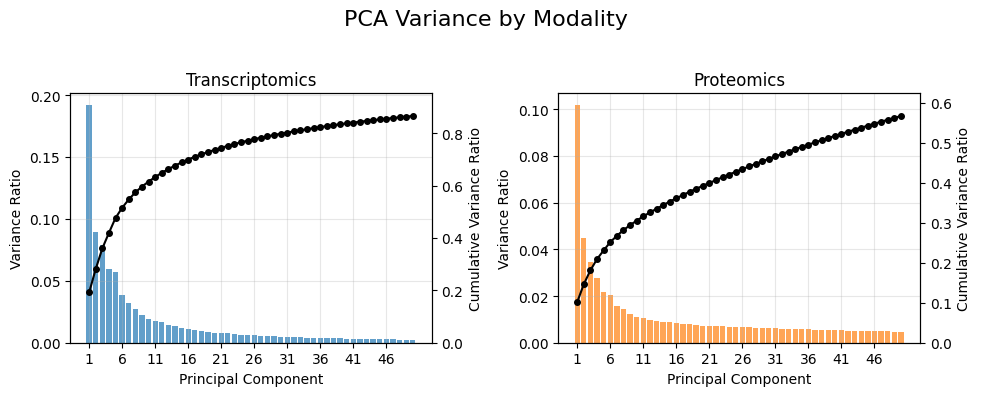
The scree plots show that variance is distributed across many components instead of being concentrated in just a few. The gradual decline — with no sharp “elbow” — indicates the presence of multiple sources of variation rather than a small number of dominant factors. This pattern is typical of patient-derived samples, which exhibit both genetic and environmental heterogeneity.

To identify the major observed sources of variation — biological or technical — I will calculate correlations between principal components and sample attributes.

# put these at the top regardless of significance
PRIORITIZED_PHENOTYPES = ["date_freezing", "proteomics_runorder", "case", "responsive_to_acute_treatment", "OHCblPlus", "MMA_urine"]

results = mdata_eda.analyze_pc_metadata_correlation_mudata(
    mdata,
    n_pcs=8,
    prioritized_vars=PRIORITIZED_PHENOTYPES,  # This will always show 'case' variable at the top
    pca_kwargs={'svd_solver': 'arpack'},
    figsize = (12, 7)
)

plt.show()

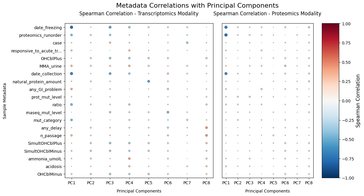
The PCA analysis reveals several key patterns. Batch effects dominate the primary sources of variation — date_freezing and proteomics_runorder show stronger associations with the leading PCs than disease variables, highlighting the importance of including them as covariates. Disease signals are subtle; the weak correlations between disease markers and PCs suggest that, like its variable clinical presentation, MMA is also molecularly heterogeneous. Finally, proteomics_runorder strongly affects proteomics data but not transcriptomics.

This analysis informs my regression model specification: I will use different covariates for each data modality based on the identified batch effects.

Supervised analysis

I can now systematically identify molecular features associated with disease phenotypes, including case–control status, responsiveness to acute treatment, OHCblPlus (enzyme activity), and urine MMA levels. To do this, I will use Generalized Additive Models (GAMs) to account for potentially nonlinear effects of date_freezing and proteomics_runorder on feature abundance.

My modeling strategy involves feature-wise testing, where each gene or protein is independently analyzed through regression models that capture specific biological effects while adjusting for covariates. For transcripts, I control for date_freezing; for proteins, I control for both date_freezing and proteomics_runorder (I will later validate that including both is appropriate). Finally, I apply false discovery rate (FDR) control to account for multiple testing across all features (see my lFDR shrinkage post for a detailed review).

Forny et al., approached this problem by regressing feature-level abundances on OHCblPlus while accounting for genetic-relatedness of individuals using random effects. This is especially important in rare disease settings where multiple cases and controls often come from the same family. Since genotypes are protected medical information under Switzerland’s Federal Act on Data Protection (FADP), this information wasn’t available for my re-analysis.

# Process each modality
regression_results = list()
for modality in mdata.mod_names:
    
    modality_results = list()
    # Apply regression per feature
    for formula_name, formula in REGRESSION_FORMULAS[modality].items():

        summaries = adata_regression.adata_model_fitting(
            mdata[modality],
            formula,
            n_jobs=4,
            layer = ANALYSIS_LAYER,
            model_name = formula_name,
            progress_bar = False
        )

        # Remove intercepts and covariates
        mask = [name == term for name, term in zip(summaries["model_name"], summaries["term"])]
        summaries = summaries.iloc[mask]

        modality_results.append(summaries)
    
    # combine results and add modality first
    modality_results = pd.concat(modality_results).assign(modality = modality)[['modality'] + [col for col in pd.concat(modality_results).columns if col != 'modality']]
    
    # add results to adata's modality-level var table
    adata_regression.add_regression_results_to_anndata(
        mdata[modality],
        modality_results,
        inplace = True
    )
    
    regression_results.append(modality_results)

regression_results_df = pd.concat(regression_results)

create_stacked_barplot_from_regression(regression_results_df)
plt.show()

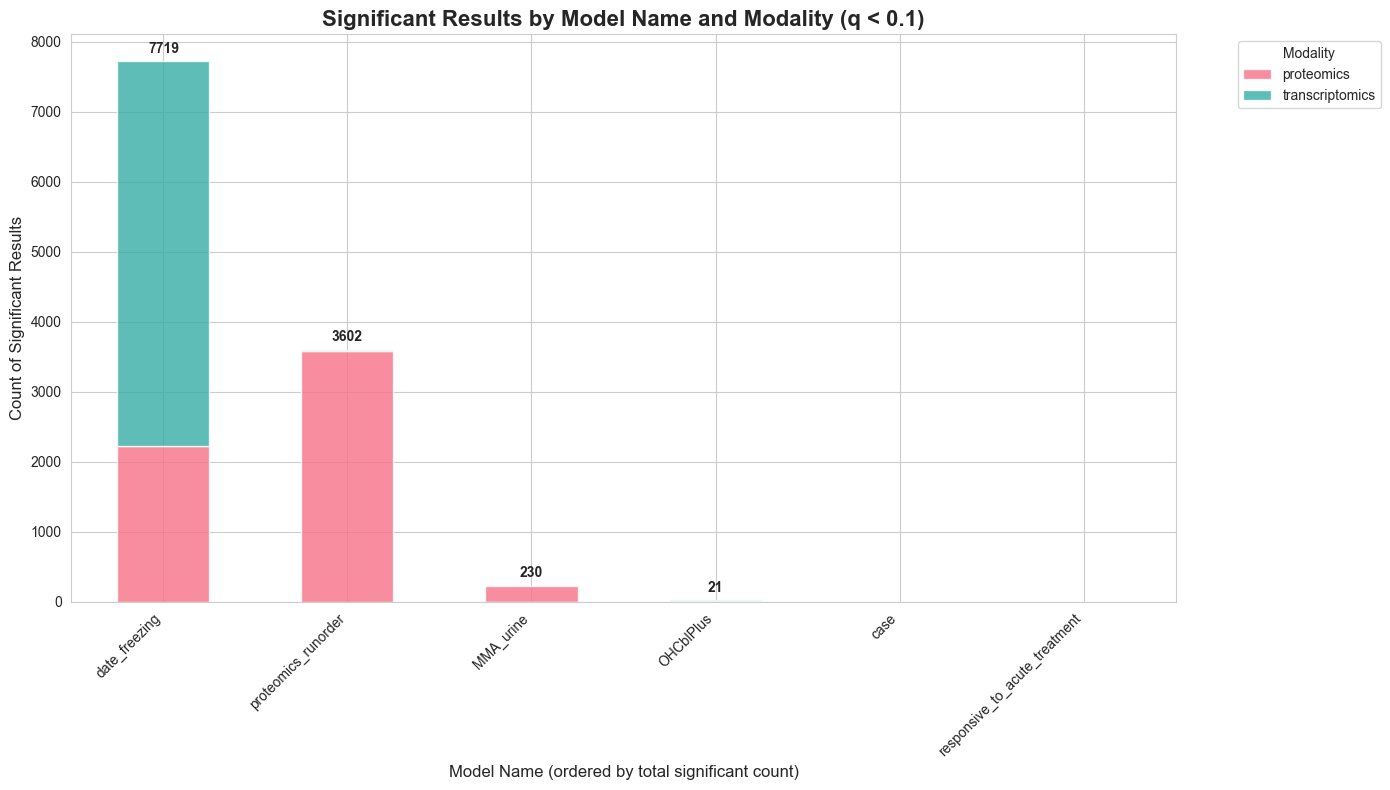
The batch effect validation confirms my modeling strategy: when fitting a model with both proteomics_runorder and date_freezing to both modalities, I observe significant associations for both covariates in the proteomics data, while runorder shows no effect in the transcriptomics data—confirming that this is indeed a proteomics-specific technical artifact. Although the overall number of nominally significant associations appears modest for most biological effects of interest, the p-value histograms — as you will see—suggest that this reflects limitations in statistical power rather than an absence of biological signal. This highlights an important opportunity for network-based methods, which can potentially recover weak but mechanistically coherent associations by pooling signals across connected molecular components, rather than analyzing features in isolation.

To break ground on this problem, I asked Claude to draft a differential expression workflow that accepts an AnnData object and a regression formula as input, and outputs broom-like tidy summaries for each feature-by-term combination (term, effect size, t-statistic, p-value). Claude quickly produced a working example with some nice features, such as parallelization. However, the actual implementation amounted to spaghetti code. Under the hood, the functions ignored the provided formulas and instead reformulated them as a set of simple linear regressions. This approach mishandled covariates, and the large gap between my intent—as someone with a fair bit of statistical knowledge—and the actual implementation was concerning.

There was no easy fix, and it didn’t make sense to build a proper statistical framework from a collection of loosely connected .py files lacking tests. So, I sidestepped the issue and implemented the workflow in my shackett-utils package as feature-level OLS and GAM modules, a multi-model fitting module, and a lightweight wrapper that specifically supports AnnData as input.

To flesh out these modules, I collaborated extensively with Claude — particularly on writing tests. Claude was especially helpful in implementing tricky features, such as calculating p-values in log-space to avoid underflow to zero.

This vignette nicely encapsulates my experience doing science with AI. It’s excellent for breaking ground on a problem and for tasks that are either easily verifiable (like visualization) or routine (like exploratory data analysis). For such one-off tasks, AI is probably sufficient. But for problems where the implementation strategy is unclear, it’s important to approach the work like traditional software development: implement specific features, write tests consistently, and avoid feature bloat. In this context, AI can be a powerful asset — implementing features and tests in real time — while allowing us humans to focus on providing code review.

Interpreting p-value histograms

# plot p-value histograms
TERMS_FOR_PVALUE_HISTOGRAM = ["case", "responsive_to_acute_treatment", "MMA_urine", "OHCblPlus", "date_freezing"]
stats_viz.plot_pvalue_histograms(
    regression_results_df.query("term in @TERMS_FOR_PVALUE_HISTOGRAM"),
    term_column = "term",
    fdr_cutoff = FDR_CUTOFF
)
plt.show()

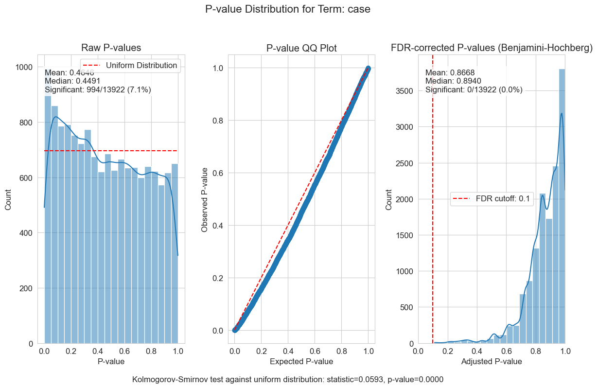
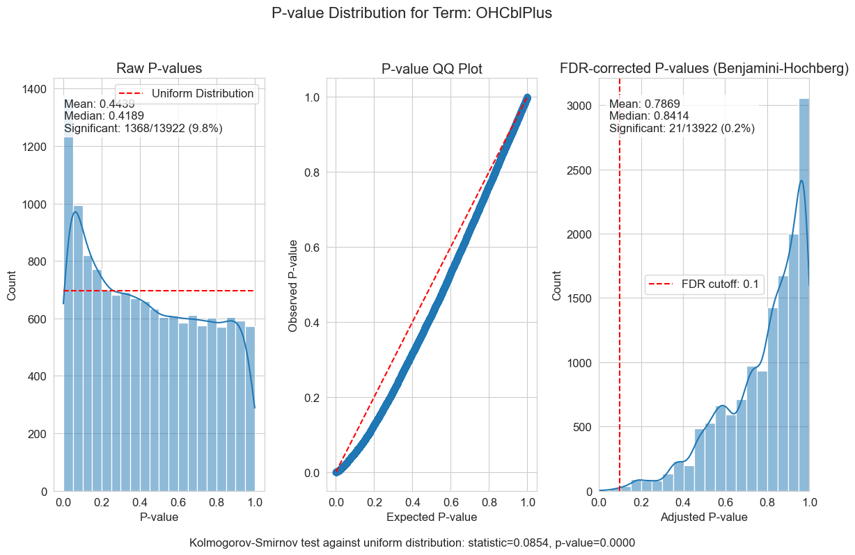
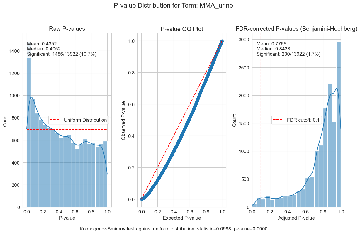
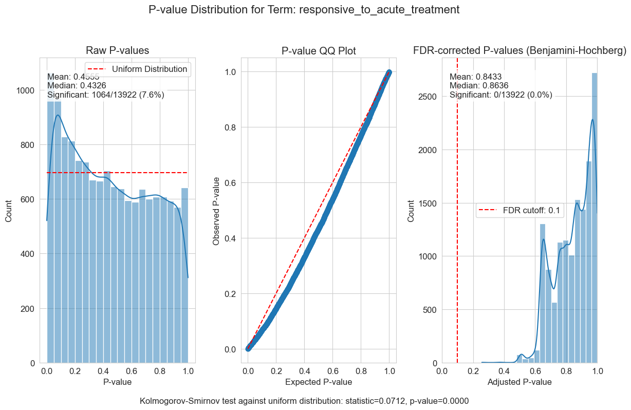
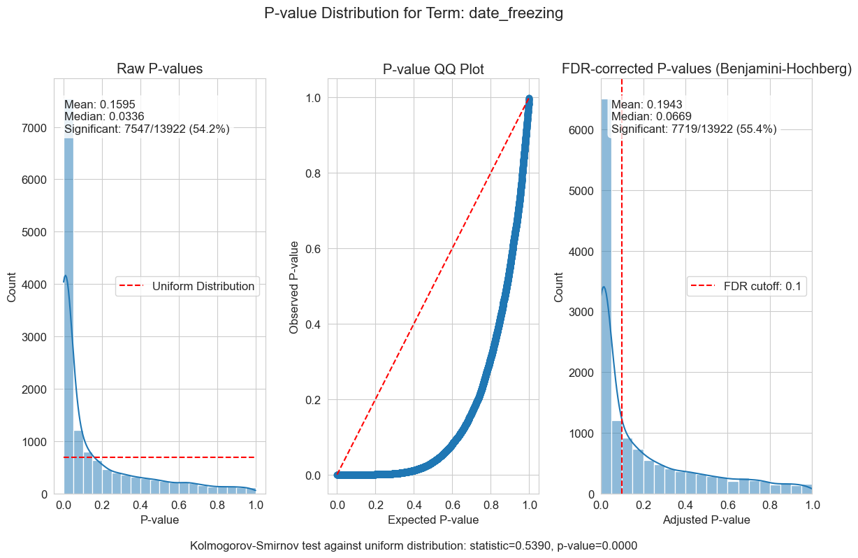
P-value distributions provide powerful diagnostics for my regression models. You can think of a p-value histogram as a mixture of two distributions: a Uniform(0,1) distribution representing true null hypotheses, and a distribution skewed toward zero representing true positives. Visually examining this mixture helps estimate the proportion of real signals and detect pathological features, such as p-value clumping or enrichment near 1.

My results show varying levels of biological signal across different phenotypes: MMA_urine and OHCblPlus display clear evidence of biological associations, whereas case status shows little signal after covariate adjustment.

Validating results: focus on MMUT

Before moving forward, it’s important to verify that my models are capturing true biological signals by spot-checking some gold-standard associations. Let’s examine the top associations and confirm that they make biological sense, focusing on MMUT (UniProt: P22033), the primary gene involved in MMA pathogenesis.

PHENOTYPE_EXAMPLE = ["MMA_urine", "OHCblPlus"]

for phenotype in PHENOTYPE_EXAMPLE:
    example_stat_summaries = mdata["proteomics"].var.loc[:, mdata["proteomics"].var.columns.str.contains(phenotype)].sort_values(f"log10p_{phenotype}").head()
    
    display(HTML(f"<h4>Top associations with {phenotype}</h4>"))
    display(napistu_utils.style_df(example_stat_summaries))

Top associations with MMA_urine

            est_MMA_urine   p_MMA_urine   log10p_MMA_urine   q_MMA_urine   stat_MMA_urine   stderr_MMA_urine
  --------- --------------- ------------- ------------------ ------------- ---------------- ------------------
  uniprot                                                                                    
  P22033    -0.207          0.000         -8.239             0.000         -6.077           0.034
  O43617    0.072           0.000         -6.295             0.001         5.187            0.014
  O75976    -0.135          0.000         -5.239             0.009         -4.655           0.029
  Q9UJW0    0.086           0.000         -5.061             0.010         4.561            0.019
  O43237    0.057           0.000         -4.999             0.010         4.528            0.013

Top associations with OHCblPlus

            est_OHCblPlus   p_OHCblPlus   log10p_OHCblPlus   q_OHCblPlus   stat_OHCblPlus   stderr_OHCblPlus
  --------- --------------- ------------- ------------------ ------------- ---------------- ------------------
  uniprot                                                                                    
  P61106    0.070           0.000         -5.308             0.014         4.691            0.015
  P22033    0.283           0.000         -5.221             0.014         4.645            0.061
  Q13428    0.123           0.000         -4.033             0.090         3.987            0.031
  P32119    -0.099          0.000         -3.939             0.090         -3.931           0.025
  Q7L0Y3    0.224           0.000         -3.849             0.090         3.877            0.058

GENE_ASSOCIATIONS = {
    "transcriptomics" : "ENSG00000146085",
    "proteomics" : "P22033"
}

for modality, identifier in GENE_ASSOCIATIONS.items():

    gene_summaries = mdata[modality].var.loc[mdata[modality].var_names.str.contains(identifier)]
    df_transposed = gene_summaries.T.reset_index()
    df_transposed.columns = ['column', 'value']  # Rename columns
    if modality == "proteomics":
        # remove entries starting with PG.
        df_transposed = df_transposed[~df_transposed["column"].str.startswith("PG.")]

    # Extract the prefix and term from the column names
    df_transposed['prefix'] = df_transposed['column'].str.extract(r'^([^_]+)_')
    df_transposed['term'] = df_transposed['column'].str.extract(r'^[^_]+_(.+)$')

    # Pivot to get prefixes as columns and terms as rows
    df_pivoted = df_transposed.pivot(index='term', columns='prefix', values='value')

    display(HTML(f"<h4>Top associations with {modality} {identifier}</h4>"))
    display(napistu_utils.style_df(df_pivoted))

Top associations with transcriptomics ENSG00000146085

  prefix                          est      log10p   p       q       stat     stderr
  ------------------------------- -------- -------- ------- ------- -------- --------
  term                                                                        
  MMA_urine                       -0.038   -0.378   0.418   0.873   -0.811   0.046
  OHCblPlus                       0.383    -6.451   0.000   0.003   5.261    0.073
  case                            -0.606   -1.622   0.024   0.627   -2.275   0.266
  date_freezing                   nan      nan      0.922   0.927   nan      nan
  proteomics_runorder             nan      nan      0.820   0.973   nan      nan
  responsive_to_acute_treatment   -0.210   -0.666   0.216   0.756   -1.242   0.169

Top associations with proteomics P22033

  prefix                          est      log10p   p       q       stat     stderr
  ------------------------------- -------- -------- ------- ------- -------- --------
  term                                                                        
  MMA_urine                       -0.207   -8.239   0.000   0.000   -6.077   0.034
  OHCblPlus                       0.283    -5.221   0.000   0.014   4.645    0.061
  case                            -0.187   -0.423   0.378   0.895   -0.884   0.211
  date_freezing                   nan      nan      0.560   0.667   nan      nan
  proteomics_runorder             nan      nan      0.013   0.022   nan      nan
  responsive_to_acute_treatment   -0.349   -2.067   0.009   0.512   -2.654   0.131

The regression analysis successfully identified expected biological relationships, providing confidence in my approach. As anticipated, MMUT showed strong associations with both the MMA_urine and OHCblPlus biomarkers. Notably, MMUT exhibited stronger associations with protein levels for MMA_urine, but with both transcript and protein levels for OHCblPlus, suggesting different underlying biological mechanisms.

The association patterns reveal distinct regulatory mechanisms. OHCblPlus correlates with both MMUT protein and transcript levels, consistent with genetic defects impacting transcription—likely through mutations affecting transcription or causing nonsense-mediated decay—which in turn result in depleted protein levels and reduced enzymatic activity. In contrast, the association of MMA_urine with MMUT protein levels—but not with its transcripts—suggests that translational and/or post-translational regulation of MMUT plays a major role in influencing its metabolic impact.

This disconnect between transcript levels and metabolic outcomes could be key to understanding idiopathic MMA cases. The selective correlation with protein levels indicates that MMUT function depends not only on gene expression but also on post-transcriptional regulatory networks that modulate protein stability, localization, or activity. Understanding these mechanisms could help uncover the etiology underlying cases without clear genetic explanations.

This makes urine MMA particularly valuable as an integrated readout of disease pathophysiology, rather than merely a simple marker of enzyme deficiency.

Unsupervised analysis

Unsupervised analyses help to identify patterns in the data with minimal assumptions about what should be important. Factor analysis is particularly intuitive for genomics data because it describes cellular states through gene expression programs—coordinated changes in related genes that reflect underlying biological processes.

Multi-Omic Factor Analysis (MOFA) extends this concept to multimodal data by discovering the principal sources of variation across different data types. Rather than concatenating features and treating transcripts and proteins equivalently, MOFA disentangles axes of heterogeneity shared across multiple modalities from those specific to individual data types. This will allow me to determine whether certain biological programs create coordinated responses across transcriptomics and proteomics or manifest differently in each modality.

Each factor represents a biological or technical program with two key components: loadings (which features participate in the program) and usages (how much each sample expresses the program). MOFA requires selecting the optimal number of factors — too few factors miss important biological programs, while too many introduce noise and overfitting. I will systematically test different numbers of factors to select an optimal value that balances variance explained and factor interpretability.

# update the MuData object so `nvars` and `nobs` are appropriate
intersected_mdata = md.MuData({k: v for k, v in mdata.mod.items()})

muon.pp.intersect_obs(intersected_mdata)  # This modifies mdata in-place

# Run the factor scan
results_dict = mdata_factor_analysis.run_mofa_factor_scan(
    intersected_mdata, 
    factor_range=FACTOR_RANGE,
    use_layer=ANALYSIS_LAYER,  # Adjust to your normalized layer
    models_dir=MOFA_PARAM_SCAN_MODELS_PATH,
    overwrite=OVERWRITE
)

# Extract variance metrics from all models
metrics = mdata_factor_analysis.calculate_variance_metrics(results_dict)

mdata_factor_analysis.visualize_factor_scan_results(metrics, user_factors=OPTIMAL_FACTOR)
plt.show()

    Optimal number of factors based on different criteria:
      Elbow method: 10 factors
      Threshold method: 48 factors
      Balanced method: 24 factors
      User-specified: 30 factors

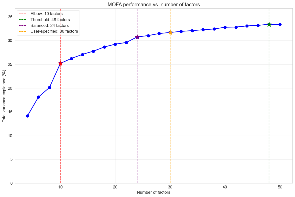
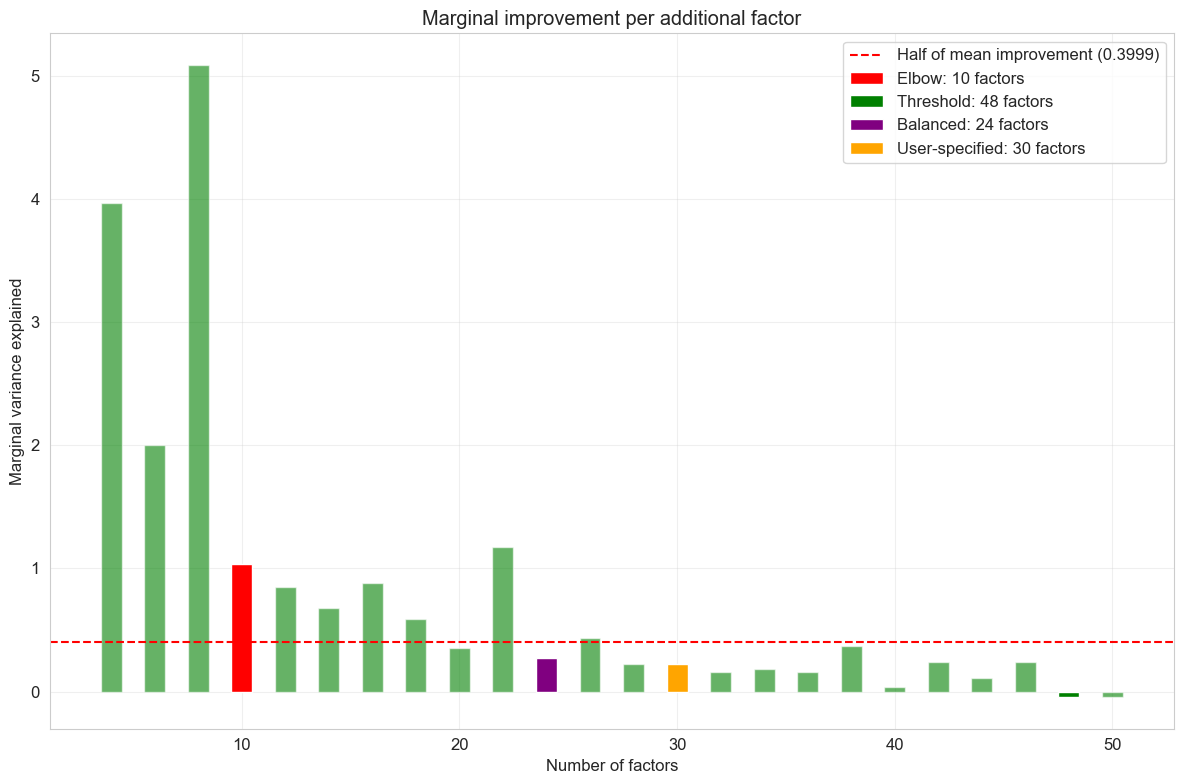
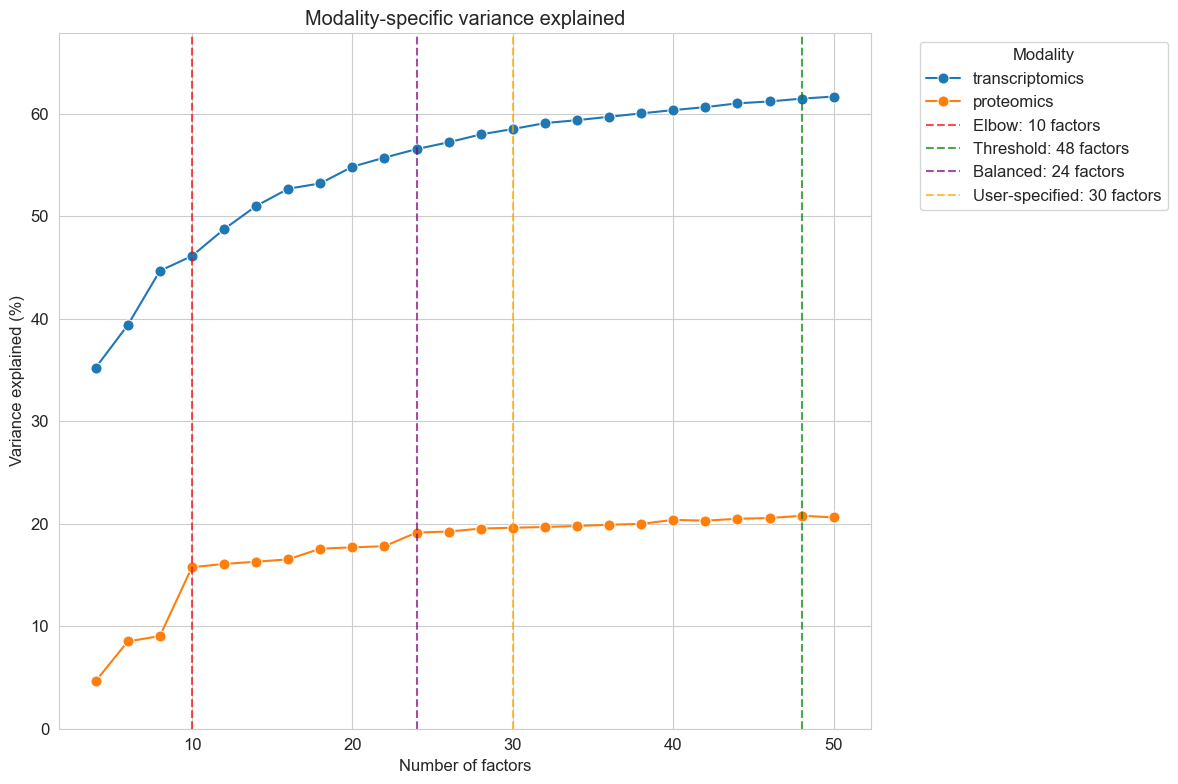
The factor scan results help me identify the optimal model complexity. I look for the point where adding more factors yields diminishing returns in variance explained while avoiding overfitting that would reduce factor interpretability.

Claude did well organizing the hyperparameter scan and implementing various approaches for selecting the optimal number of factors (K). While I wasn’t particularly impressed with the specific model selection criteria it chose, this didn’t matter much in practice. Factor analyses like MOFA exhibit diminishing returns, where later factors tend to have smaller, sparser loadings and capture less meaningful variation. This means the overall results are relatively robust to the exact choice of K, as long as it falls within a reasonable range.

With 30 factors selected as optimal, I can fit the final MOFA model and examine the distributions of the factors:

if not os.path.isfile(OPTIMAL_MODEL_H5MU_PATH) or OVERWRITE:

    optimal_model = mdata_factor_analysis.create_minimal_mudata(
        intersected_mdata,
        include_layers=[ANALYSIS_LAYER],
        include_obsm=True,
        include_varm=True
    )

    mdata_factor_analysis._mofa(
        optimal_model,
        n_factors=OPTIMAL_FACTOR,
        use_obs=None,
        use_var=None,
        use_layer=ANALYSIS_LAYER,
        convergence_mode="medium",
        verbose=False,
        save_metadata=True
    )

    md.write_h5mu(OPTIMAL_MODEL_H5MU_PATH, optimal_model)
else:
    optimal_model = md.read_h5mu(OPTIMAL_MODEL_H5MU_PATH)
    
mdata_factor_analysis.plot_mofa_factor_histograms(optimal_model)
plt.show()

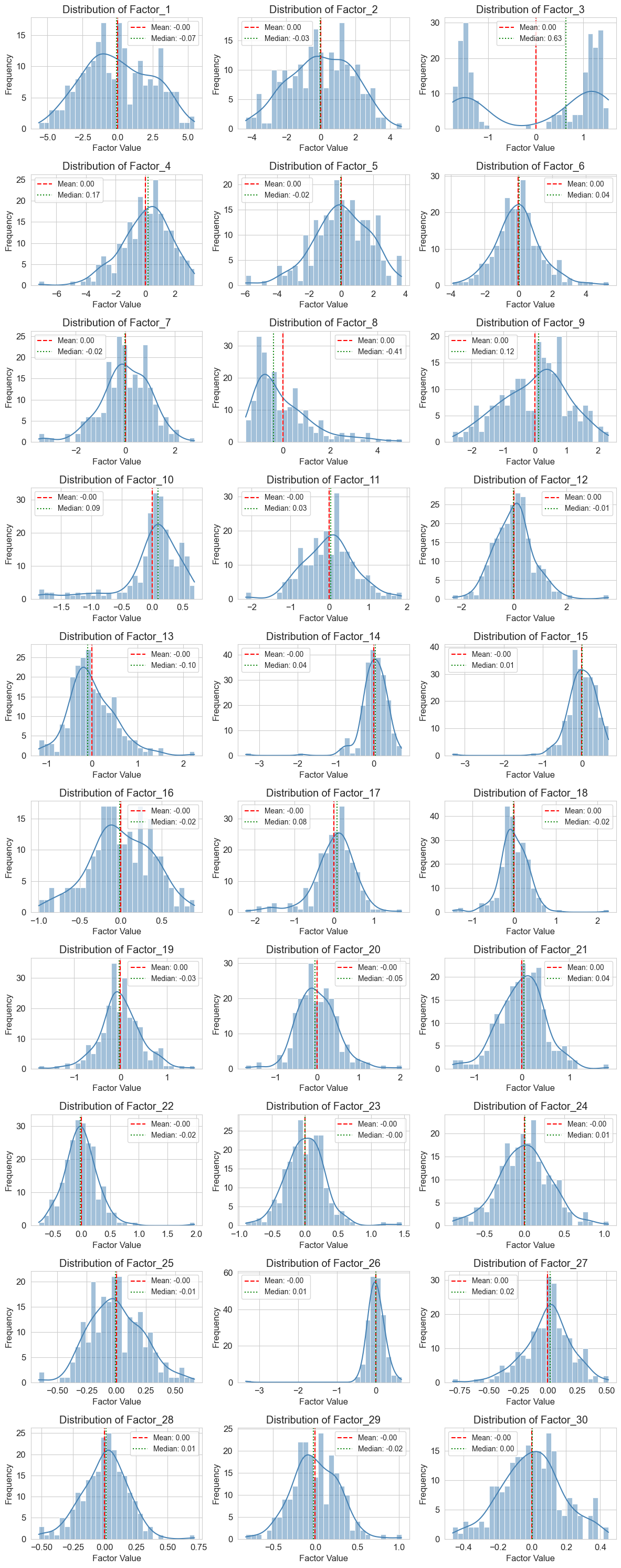
With 30 factors extracted, I aim to identify those that capture disease biology versus technical variation or normal biological heterogeneity. To do this, I’ll apply the same regression approach used for individual features, testing whether factor usages (how much each sample expresses each factor) correlate with disease phenotypes such as MMA_urine levels and treatment responsiveness. Covariates are less of a concern here because different biological and technical effects are generally captured in separate components — one of the key strengths of factor analysis is its ability to account for both observed and latent confounding variables.

Factors that show significant associations across multiple disease measures, explain substantial variance in disease severity, and contain biologically coherent gene/protein sets will be my primary targets for network analysis—these represent coordinated disease programs that I can trace back to their regulatory origins.

# Apply regression per factor
factor_regressions = list()
for formula_name, formula in REGRESSION_FORMULAS["proteomics"].items():

    # Run regression analysis
    regression_results = mdata_factor_analysis.regress_factors_with_formula(
        optimal_model,
        formula=formula,
        factors=None,  # Use all factors
        progress_bar=False
    ).assign(formula_name = formula_name)

    factor_regressions.append(regression_results)
    
    # Generate summary table
    summary_table = mdata_factor_analysis.summarize_factor_regression(
        regression_results,
        alpha=FDR_CUTOFF,
        group_by_factor=False
    ).query(f"term == '{formula_name}'")

    if summary_table.shape[0] > 0:

        display(HTML(f"\n<h4>Factors associated with {formula_name}</h4>\n"))
        display(napistu_utils.style_df(summary_table))

factor_regressions_df = pd.concat(factor_regressions)
optimal_model.uns["factor_regressions"] = factor_regressions_df

Factors associated with case

       factor_name   term   estimate   standard_error   statistic   p_value    q_value
  ---- ------------- ------ ---------- ---------------- ----------- ---------- ----------
  36   Factor_10     case   0.207      0.052            3.992       9.22e-05   2.77e-03
  32   Factor_9      case   -0.650     0.236            -2.756      6.39e-03   9.58e-02

Factors associated with MMA_urine

       factor_name   term        estimate   standard_error   statistic   p_value    q_value
  ---- ------------- ----------- ---------- ---------------- ----------- ---------- ----------
  28   Factor_8      MMA_urine   -0.150     0.045            -3.342      9.92e-04   2.98e-02
  8    Factor_3      MMA_urine   0.040      0.014            2.814       5.38e-03   5.94e-02
  36   Factor_10     MMA_urine   0.025      0.009            2.781       5.94e-03   5.94e-02
  60   Factor_16     MMA_urine   0.038      0.015            2.600       1.00e-02   7.51e-02

Factors associated with proteomics_runorder

       factor_name   term                  p_value    q_value
  ---- ------------- --------------------- ---------- ----------
  6    Factor_3      proteomics_runorder   1.11e-16   1.67e-15
  27   Factor_10     proteomics_runorder   1.11e-16   1.67e-15
  39   Factor_14     proteomics_runorder   3.37e-07   3.37e-06
  21   Factor_8      proteomics_runorder   5.79e-04   4.34e-03
  69   Factor_24     proteomics_runorder   1.51e-02   7.87e-02
  12   Factor_5      proteomics_runorder   1.57e-02   7.87e-02

Factors associated with date_freezing

       factor_name   term            p_value    q_value
  ---- ------------- --------------- ---------- ----------
  1    Factor_1      date_freezing   6.29e-13   1.89e-11
  88   Factor_30     date_freezing   2.52e-05   3.41e-04
  22   Factor_8      date_freezing   3.41e-05   3.41e-04
  49   Factor_17     date_freezing   1.13e-04   8.48e-04
  55   Factor_19     date_freezing   2.69e-04   1.62e-03
  31   Factor_11     date_freezing   4.07e-04   2.03e-03
  46   Factor_16     date_freezing   8.81e-04   3.77e-03
  37   Factor_13     date_freezing   6.41e-03   2.40e-02
  64   Factor_22     date_freezing   9.81e-03   3.27e-02
  28   Factor_10     date_freezing   1.22e-02   3.51e-02
  52   Factor_18     date_freezing   1.36e-02   3.51e-02
  43   Factor_15     date_freezing   1.40e-02   3.51e-02
  25   Factor_9      date_freezing   1.79e-02   4.13e-02
  13   Factor_5      date_freezing   2.03e-02   4.35e-02
  67   Factor_23     date_freezing   2.17e-02   4.35e-02
  58   Factor_20     date_freezing   3.15e-02   5.90e-02
  10   Factor_4      date_freezing   4.45e-02   7.85e-02
  85   Factor_29     date_freezing   5.24e-02   8.73e-02
  79   Factor_27     date_freezing   5.64e-02   8.91e-02
  40   Factor_14     date_freezing   6.13e-02   9.08e-02
  61   Factor_21     date_freezing   6.36e-02   9.08e-02

While I generally like this approach and have seen it successfully applied to single-cell RNA-seq data using cNMF, it didn’t work particularly well for this dataset. Most disease phenotypes show only weak correlations with factor usages, similar to the feature-wise significance tests. The clearest exception is urine MMA levels, which are strongly associated with latent factor 3 (LF3). However, LF3 is bimodal and also correlated with proteomics run order and sample freezing date, so buyer beware. Curiously, case status was also associated with a couple of factors despite little feature-level signal.

The prominence of non-disease biology in my factor analysis highlights both a key strength and a limitation of the method: it is agnostic to the biology of interest and instead captures the dominant sources of variation in the data. In human disease datasets, coherent disease signatures are often distributed across many small factors rather than concentrated in a few large ones, making them harder to detect amid technical variation and biological heterogeneity.

Summary and next steps

This analysis demonstrates a systematic approach to extracting disease-relevant molecular profiles from multimodal genomics data. Using the Forny et al. MMA dataset, I have shown how careful data processing, covariate adjustment, and the use of both supervised and unsupervised methods can reveal subtle but biologically meaningful disease signals.

Methodological insights:

• scverse integration: Demonstrated how organizing multimodal data using AnnData/MuData containers facilitates reproducible analysis while maintaining seamless integration with the broader genomics ecosystem.

• Modality-specific covariate modeling: PCA revealed that batch effects (proteomics run order, sample freezing dates) impacted transcriptomics and proteomics data differently, enabling tailored regression models for each modality that improved my statistical power for detecting biological signals.

• AI-assisted development workflow: Large language models (LLMs) proved effective for rapid prototyping and handling complex visualization syntax (e.g., matplotlib), but encountered serious issues with statistical implementation — initially producing spaghetti code that silently converted multiple regressions into simple regressions. The solution was to treat AI as a development collaborator, following software engineering best practices by implementing specific features with tests in a structured Python package rather than relying on AI for end-to-end development.

Biological insights:

• MMUT regulatory patterns: Different association patterns between transcript and protein levels suggest that translational or post-translational control mechanisms shape metabolic impact, potentially explaining idiopathic MMA cases.

• Biomarker performance: Urine MMA showed stronger statistical associations with molecular features than traditional enzyme activity measures, suggesting it captures integrated disease pathophysiology beyond simple enzyme deficiency.

• Disease heterogeneity: Weak PCA associations with disease status mirror the clinical heterogeneity observed in MMA patients, confirming that molecular signatures reflect the complex and variable nature of disease presentation.

Transitioning to network analysis

While my statistical approach successfully identified disease-associated molecular programs, interpreting their biological significance requires additional context. These molecular signatures represent starting points for deeper mechanistic investigation. In part two, I will map these statistical associations onto genome-scale biological networks using Napistu. This approach will trace disease signals from downstream molecular effects to potential upstream regulatory causes, converting statistical associations into testable biological hypotheses.