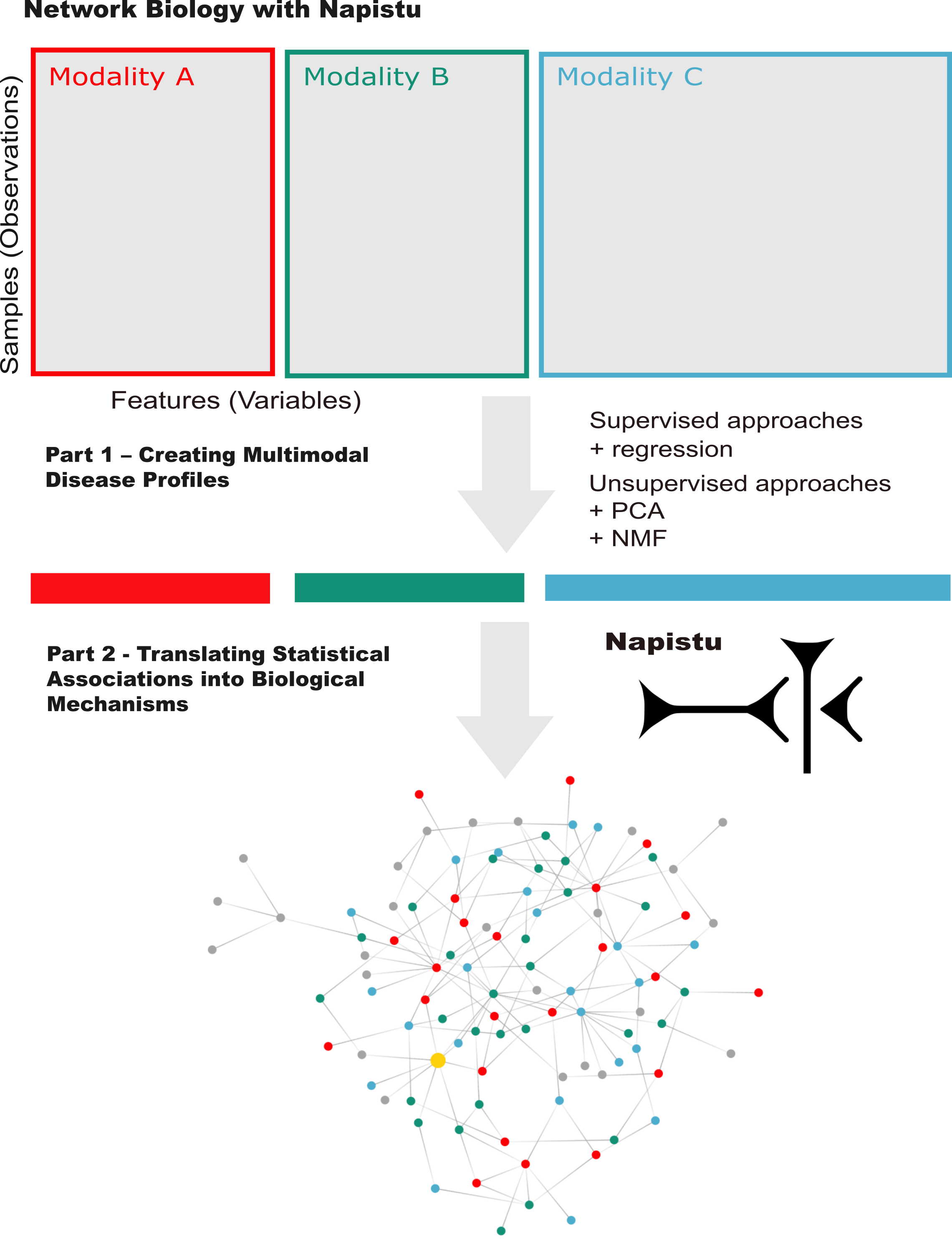
Network Biology with Napistu, Part 2: Translating Statistical Associations into Biological Mechanisms

This is part two of a two-part series on Napistu — a new framework for building genome-scale molecular networks and integrating them with high-dimensional data. Using a methylmalonic acidemia (MMA) multimodal dataset as a case study, I’ll demonstrate how to distill disease-relevant signals into mechanistic insights through network-based analysis.

From statistical associations to biological mechanisms

Modern genomics excels at identifying disease-associated genes and proteins through statistical analysis. Methods like Gene Set Enrichment Analysis (GSEA) group these genes into functional categories, offering useful biological context. However, we aim to go beyond simply identifying which genes and gene sets change. Our goal is to understand why these genes change together, uncovering the mechanistic depth typically seen in Figure 1 of a Cell paper. To achieve this, we must identify key molecular components, summarize their interactions, and characterize the dynamic cascades that drive emergent biological behavior.

In this post, I’ll demonstrate how to gain this insight by mapping statistical disease signatures onto genome-scale biological networks. Then, using personalized PageRank, I’ll trace signals from dysregulated genes back to their shared regulatory origins. This transforms lists of differentially expressed genes into interconnected modules that reveal upstream mechanisms driving coordinated molecular changes.

Napistu’s implementation

Napistu makes network biology practical through three core capabilities:

1. Pathway representation with SBML_dfs

   Napistu uses a custom format, SBML_dfs, to faithfully capture regulatory mechanisms. It tracks genes, metabolites, protein complexes, and drugs as molecular species, connecting them through regulatory interactions and biochemical transformations.

2. Translation to NapistuGraphs

   It provides tools to convert these pathway representations into NapistuGraph, where vertices represent molecular species and edges represent direct regulatory relationships.

3. Biological query capabilities

   Napistu enables users to ask general-purpose questions of these networks, such as:

   • What is the relationship between two genes?
   • What are the direct and indirect regulators of a molecular target?
   • And — as we’ll explore in this post — what shared mechanisms unite a set of disease-associated genes?

Throughout this post, I’ll use two types of asides to add context without interrupting the main flow:

• 🟩 Green boxes offer biological background and systems biology “inside baseball.”
• 🟦 Blue boxes share reflections on building scientific software in the age of AI.

For biologists: Discover a versatile open-source framework designed to tackle one of the key final mile problems when working with high-dimensional genomics data. I’ll show you how network propagation recovers both the genetic drivers of MMA and its major metabolic dysfunction from functional changes in the transcriptome and proteome. This regulation suggests that investigating specific regulatory pathways involved in metabolic sensing — such as ROS and sirtuins — could offer promising insights into MMA pathophysiology.

For computational folks: In this post, I’ll walk you through how Napistu seamlessly integrates network models with high-dimensional data using practical workflows — from multimodal identifier mapping to personalized PageRank with empirical nulls. Plus, I’ll share firsthand insights on leveraging AI to develop complex scientific software — tackling challenges that often lie beyond the reach of large language models (LLMs).

Series overview

Part 1: Creating Multimodal Disease Profiles established the foundation for this post by systematically extracting disease-relevant molecular signatures from the Forny et al. methylmalonic acidemia dataset. Through careful batch effect correction and both supervised and unsupervised analyses, I uncovered coordinated gene and protein expression programs linked to key disease phenotypes. The result? Clean, quantitative profiles — ready for network-level mechanistic exploration. Most profiles were generated using Generalized Additive Models (GAMs), each combining regression summaries (effect size, statistic, p/q-value) with phenotypes — such as case vs. control, MMA urine levels reflecting metabolic burden, or OHCblPlus as a proxy for enzyme activity.

In this post, I’ll decode these statistical signals by mapping them onto genome-scale biological networks with Napistu. The goal is to trace disease signals from dysregulated genes and proteins upstream to their common regulatory drivers. I’ll begin by mapping statistical results onto genes within the pathway model, then transfer these signals to nodes in a regulatory graph. Finally, using personalized PageRank with empirical null models, I’ll identify subgraphs enriched for disease signals — revealing the upstream regulatory mechanisms driving MMA pathophysiology.

Integrating genome-scale networks and genome-wide data

Environment setup

To reproduce this analysis:

1. Follow the setup instructions and run the first notebook in the series creating_multimodal_profiles.qmd. This will set up both the Python environment and the input data required for this analysis.

2. Download the napistu_network_propagation.qmd notebook

3. Modify the following code block in your copy of the notebook to set appropriate paths:

   a. CACHE_DIR should match the value used in creating_multimodal_profiles.qmd b. INPUT_DATA_DIR should be a suitable location for saving the network representations (~4 GB in size)

4. Run the notebook and render an HTML output by executing:

   quarto render napistu_network_propagation.qmd
   

First, I’ll load the necessary Python modules, configure file paths, set global parameters, and define utility functions.

import os
import re
from pathlib import Path
from types import SimpleNamespace

import mudata as md
import numpy as np
import pandas as pd
import seaborn as sns
import matplotlib.pyplot as plt
from IPython.display import display, HTML

from napistu import utils as napistu_utils
from napistu.sbml_dfs_core import SBML_dfs
from napistu.network.ng_core import NapistuGraph
from napistu.source import unnest_sources
from napistu.gcs import downloads
from napistu.matching import mount
from napistu.network import net_propagation
from napistu.network import data_handling
from napistu.network import ng_utils
from napistu.scverse.loading import prepare_anndata_results_df
from napistu.scverse.loading import prepare_mudata_results_df
from napistu.constants import ONTOLOGIES, MINI_SBO_TO_NAME

from shackett_utils.statistics import hypothesis_testing
from shackett_utils.statistics import multi_model_fitting
from shackett_utils.blog.html_utils import display_tabulator
from shackett_utils.utils.pd_utils import format_numeric_columns

# setup logging
import logging
logging.basicConfig(level=logging.INFO)
logger = logging.getLogger(__name__)
logging.getLogger('matplotlib.font_manager').setLevel(logging.WARNING)
logging.getLogger('matplotlib.pyplot').setLevel(logging.WARNING) 

# File paths and data organization
# All input data should be placed in the SUPPLEMENTAL_DATA_DIR
# Cached results and models will be stored in CACHE_DIR

# paths
PROJECT_DIR = os.path.expanduser("~/napistu_mma_posts")
INPUT_DATA_DIR = os.path.join(PROJECT_DIR, "input")
CACHE_DIR = os.path.join(PROJECT_DIR, "cache")

# inputs
# model to download from GCS and store in NAPISTU_DATA_DIR
NAPISTU_ASSET = "human_consensus"
NAPISTU_ASSET_VERSION = "20250901"
# H5Mu file containing the optimal model from MOFA+ and regression summaries
OPTIMAL_MODEL_H5MU_OUTFILE = "mofa_optimal_model.h5mu"

# intermediate files
PPR_NULL_CACHE_OUTFILE = "ppr_null_cache.tsv"

# outputs
PPR_RESULTS_OUTFILE = "ppr_results.tsv"
SBML_DFS_W_DATA_OUTFILE = "sbml_dfs_w_data.pkl"
NAPISTU_GRAPH_W_DATA_OUTFILE = "napistu_graph_w_data.pkl"

# Paths to input/output files
OPTIMAL_MODEL_H5MU_PATH = os.path.join(CACHE_DIR, OPTIMAL_MODEL_H5MU_OUTFILE)
PPR_NULL_TMP_PATH = os.path.join(CACHE_DIR, PPR_NULL_CACHE_OUTFILE)
PPR_RESULTS_PATH = os.path.join(PROJECT_DIR, PPR_RESULTS_OUTFILE)
SBML_DFS_W_DATA_PATH = os.path.join(PROJECT_DIR, SBML_DFS_W_DATA_OUTFILE)
NAPISTU_GRAPH_W_DATA_PATH = os.path.join(PROJECT_DIR, NAPISTU_GRAPH_W_DATA_OUTFILE)

# dataset metadata
FORNY_MODALITIES = SimpleNamespace(
    TRANSCRIPTOMICS = "transcriptomics",
    PROTEOMICS = "proteomics"
)

MODALITIES = list(FORNY_MODALITIES.__dict__.values())

# Napistu controlled vocabulary
FORNY_ONTOLOGIES = SimpleNamespace(
    ENSEMBL_GENE = ONTOLOGIES.ENSEMBL_GENE,
    UNIPROT = ONTOLOGIES.UNIPROT
)

FORNY_DEFS = SimpleNamespace(
    # varm table names set in part
    LFS = "LFs",
    # table names used to add data sources to `sbml_dfs`
    MOFA_LFS = "mofa_lfs",
    VAR_LEVEL_RESULTS = "var_level_results",
    # template for is_X variables will be used to restrict vertex permutation
    # to measured proteins/transcripts
    INDICATOR_STR = 'is_{modality}',
    MODALITY_VAR_LEVEL_RESULTS_STR = "{modality}_var_level_results" 
)

MUDATA_ONTOLOGIES = {
    # these dicts indicate the ontology that we want to match against for each modality
    # and indicate that this ontology's identifiers are present in the .var table's index
    FORNY_MODALITIES.TRANSCRIPTOMICS :
        {
            "ontologies" : [FORNY_ONTOLOGIES.ENSEMBL_GENE],
            "index_which_ontology" : FORNY_ONTOLOGIES.ENSEMBL_GENE
        },
    FORNY_MODALITIES.PROTEOMICS :
        {
            "ontologies" : [FORNY_ONTOLOGIES.UNIPROT],
            "index_which_ontology" : FORNY_ONTOLOGIES.UNIPROT
        }
}

# attributes to use for network propagation
LFS_OF_INTEREST = ["LF1", "LF2", "LF3", "LF4", "LF5"]

# regression terms to add from var table
PPR_LINEAR_PHENOTYPES = {"MMA_urine", "OHCblPlus", "case", "responsive_to_acute_treatment"}
PPR_SMOOTH_PHENOTYPES = {"date_freezing", "proteomics_runorder"}

VAR_VARS = list()
for phenotype in PPR_LINEAR_PHENOTYPES:
    VAR_VARS.append(f"est_{phenotype}")
    VAR_VARS.append(f"stat_{phenotype}")
    # using -log10p since normal p- and q-values will underflow
    VAR_VARS.append(f"log10p_{phenotype}")
    VAR_VARS.append(f"q_{phenotype}")
for phenotype in PPR_SMOOTH_PHENOTYPES:
    VAR_VARS.append(f"q_{phenotype}")

STAT_PREFIXES = ["est", "log10p", "q", "stat"]
VAR_METADATA = pd.DataFrame([
  *[{ "phenotype" : "latent factors", "summary" : x, "variable" : x} for x in LFS_OF_INTEREST],
  *[{ "phenotype" : x, "summary" : y, "variable" : f"{y}_{x}"} for x in (PPR_LINEAR_PHENOTYPES | PPR_SMOOTH_PHENOTYPES) for y in STAT_PREFIXES if f"{y}_{x}" in VAR_VARS]
])
VAR_METADATA["summary"] = VAR_METADATA["summary"].str.replace('_', ' ')

# defining variables to add as vertex attributes and how to transform them so
# they are appropriate for personalized pagerank reset probability
ATTRIBUTES_TO_GRAPH_SPEC = [
    {
        "attribute_names": "LF",
        "table_name": FORNY_DEFS.MOFA_LFS,
        "transformation": "square"
    },
    {
        "attribute_names": "^est_",
        "table_name": FORNY_DEFS.VAR_LEVEL_RESULTS,
        "transformation": "square"
    },
    {
        "attribute_names": "^stat_",
        "table_name": FORNY_DEFS.VAR_LEVEL_RESULTS,
        "transformation": "abs"
    },
    {
        "attribute_names": "^log10p_",
        "table_name": FORNY_DEFS.VAR_LEVEL_RESULTS,
        "transformation": "negate"
    },
    {
        "attribute_names": "^q_",
        "table_name": FORNY_DEFS.VAR_LEVEL_RESULTS,
        "transformation": "underflow_guarded_nlog10"
    },
]

ATTRIBUTES_TO_GRAPH_SPEC = ATTRIBUTES_TO_GRAPH_SPEC + [{
    "attribute_names": FORNY_DEFS.INDICATOR_STR.format(modality = m),
    "table_name": FORNY_DEFS.MODALITY_VAR_LEVEL_RESULTS_STR.format(modality = m),
    "transformation": "identity"
} for m in MODALITIES]

# masks from vertex attribute name to modality to use during vertex permutation 
REGEXES_TO_MASKS = { x: FORNY_DEFS.INDICATOR_STR.format(modality = x) for x in MODALITIES }

# utility functions

def underflow_guarded_nlog10(x):
    if x < 1e-12:
        return 1e-12 # underflow guard
    else:
        return -np.log10(x)

CUSTOM_TRANSFORMATIONS = {
    # take the absolute value
    "abs" : lambda x: abs(x),
    "negate" : lambda x: -x,
    # -log10[pvalue]
    "underflow_guarded_nlog10" : underflow_guarded_nlog10,
    "square" : lambda x: x**2
}

def floor_pvalue_by_resolution(p_value, n_samples):
    """
    Floor p-values by resolution.
    """
    
    return (p_value + 1 / n_samples) * (n_samples / (n_samples + 1))

def create_stacked_barplot_seaborn(df):
    """
    Alternative version using seaborn styling
    """
    # Set seaborn style
    sns.set_style("whitegrid")
    
    # Group by measure and sum counts across modalities
    total_counts = df.groupby('variable')['count'].sum().sort_values(ascending=False)
    
    # Create pivot table
    pivot_df = df.pivot_table(index='variable', columns='modality', values='count', fill_value=0)
    pivot_df = pivot_df.reindex(total_counts.index)
    
    # Create the plot
    fig, ax = plt.subplots(figsize=(16, 8))
    
    # Use seaborn color palette
    colors = sns.color_palette("husl", len(pivot_df.columns))
    
    # Plot stacked bars
    pivot_df.plot(kind='bar', stacked=True, ax=ax, color=colors, alpha=0.8)
    
    # Customize
    ax.set_title('Stacked Barplot by Attributes and Modality', fontsize=16, fontweight='bold')
    ax.set_xlabel('Attributes (ordered by total count)', fontsize=12)
    ax.set_ylabel('Count', fontsize=12)
    ax.legend(title='Modality', bbox_to_anchor=(1.05, 1), loc='upper left')
    
    plt.xticks(rotation=45, ha='right')
    plt.tight_layout()
    plt.show()
    
    return fig, ax

def plot_ppr_enrichment_histograms(fdr_controlled_results):
    fig, axes = plt.subplots(1, 2, figsize=(8, 4), sharey=True)

    fdr_controlled_results[fdr_controlled_results["is_enriched"] == False]["p_value"].hist(
        bins=50, ax=axes[0]
    )
    axes[0].set_title("Depleted (False)")
    axes[0].set_xlabel("P-value")
    axes[0].set_ylabel("Count")

    fdr_controlled_results[fdr_controlled_results["is_enriched"] == True]["p_value"].hist(
        bins=50, ax=axes[1]
    )
    axes[1].set_title("Enriched (True)")
    axes[1].set_xlabel("P-value")

    plt.tight_layout()
    plt.show()

def reorder_by_rank_sum(df):
    """Reorder rows by sum of ranks (lower sum = better overall rank)"""
    df_num = df.replace('.', pd.NA).apply(pd.to_numeric, errors='coerce')
    max_val = df_num.max().max()
    df_filled = df_num.fillna(max_val + 1)
    rank_sums = df_filled.sum(axis=1)
    return df.loc[rank_sums.sort_values().index]

# constants affecting behavior
N_NULL_SAMPLES = 500
OVERWRITE = False

Loading MMA molecular profiles

Next, I’ll load the results generated in the previous post. These are stored in a MuData object saved as an .h5mu file. (You’ll see the contents of this object later when I discuss adding attributes to the graph.) The only modification I’ll make is adding indicator variables — is_transcriptomics and is_proteomics — to each modality to easily track measured transcripts and proteins in downstream analyses.

# lets load the Forny results so we can try adding a few different types of tables to the sbml_dfs
mdata = md.read_h5mu(OPTIMAL_MODEL_H5MU_PATH)

# create an indicator which just highlights which modalities are present in the mdata
# this will propagate this indicator to vertices in the graph which is useful for generating
# a mask for constructing vertices' null distributions
ADATA_LEVEL_VARS = dict()
for modality in MODALITIES:
    indicator_var = FORNY_DEFS.INDICATOR_STR.format(modality=modality)
    # add to var table
    mdata[modality].var[indicator_var] = 1
    # indicate that this should be added to the sbml_dfs later
    ADATA_LEVEL_VARS[modality] = [indicator_var]

Loading Napistu data

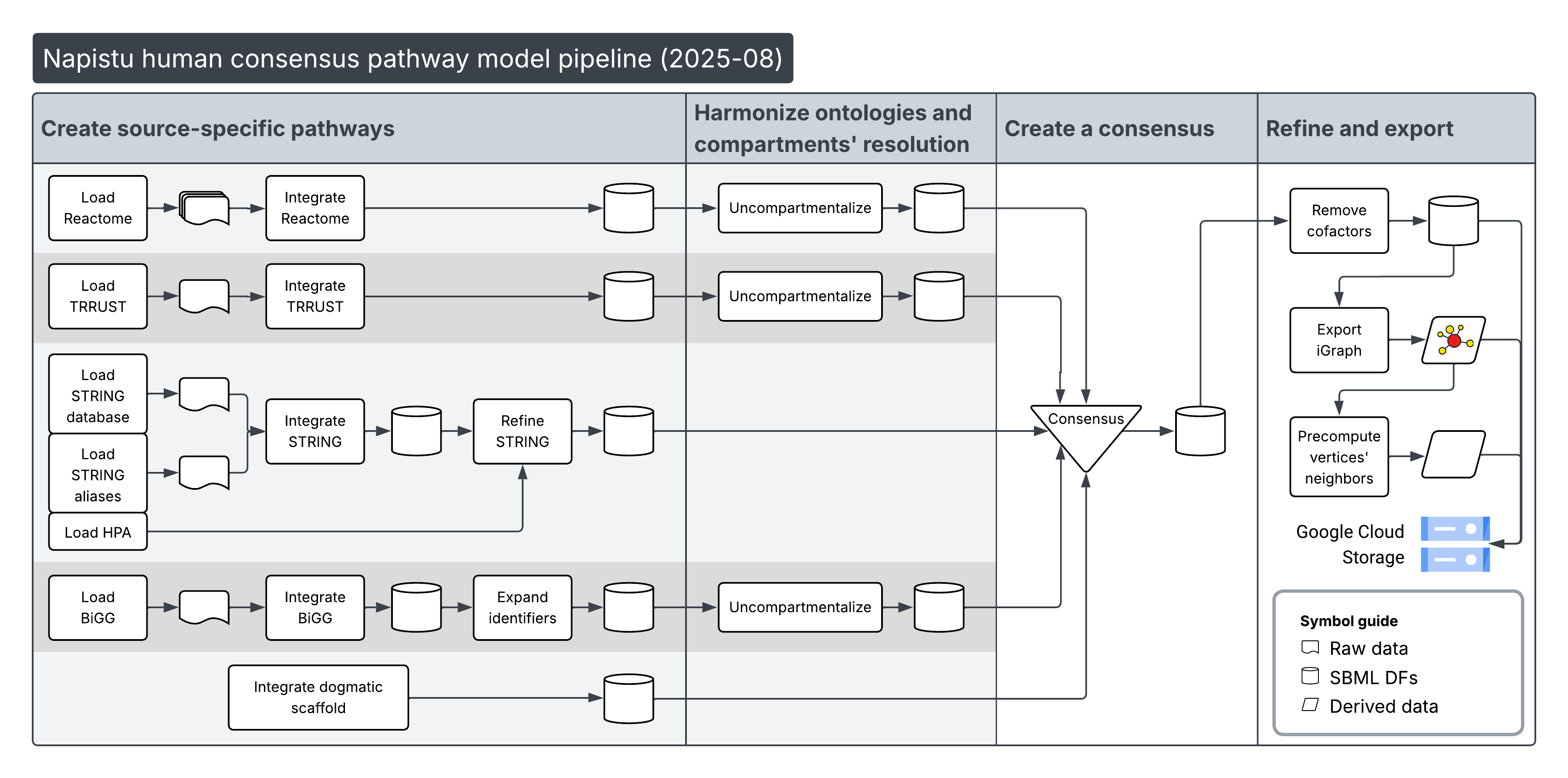
To simplify access, I’ve uploaded a lightweight test pathway (a merged set of three metabolic pathways) and the full human consensus pathway to Google Cloud Storage (GCS). These pathway representations center around two key objects:

• SBML_dfs: An in-memory relational database organizing molecular species (genes, metabolites, complexes, drugs) and their relationships (reactions, interactions).
• NapistuGraph: A directed graph representation of the same network, translating molecular species and reactions into a graph structure for downstream analysis.

The human consensus SBML_dfs and NapistuGraph I will use combine these sources:

• Reactome: human-centric gold-standard pathways of cellular physiology and signaling
• BiGG: the Recon3D genome-scale metabolic model
• TRRUST: curated transcription factor–target interactions
• STRING: undirected physical and functional interactions
• Dogma: a model of cognate relationships between genes, transcripts, and proteins with their systematic identifiers

I built this consensus using the Napistu CLI (see the build pipeline), which supports constructing and refining genome-scale pathway models for most model organisms. Below is an overview of how the human consensus was assembled:

Next, I’ll download and load the human consensus SBML_dfs from my public GCS bucket (please avoid frequent downloads 🙂), along with the corresponding NapistuGraph and a lookup table of systematic identifiers, by running:

# this will download the sbml_dfs, napistu_graph, and species_identifiers from a public GCS bucket
# or if they already exist in the INPUT_DATA_DIR, it will just set the path to the existing asset
sbml_dfs_path = downloads.load_public_napistu_asset(
    asset = NAPISTU_ASSET,
    data_dir = INPUT_DATA_DIR,
    subasset = "sbml_dfs",
    version = NAPISTU_ASSET_VERSION
)

napistu_graph_path = downloads.load_public_napistu_asset(
    asset = NAPISTU_ASSET,
    data_dir = INPUT_DATA_DIR,
    subasset = "napistu_graph",
    version = NAPISTU_ASSET_VERSION
)

species_identifiers_path = downloads.load_public_napistu_asset(
    asset = NAPISTU_ASSET,
    data_dir = INPUT_DATA_DIR,
    subasset = "species_identifiers",
    version = NAPISTU_ASSET_VERSION
)

# ~2 min load
sbml_dfs = SBML_dfs.from_pickle(sbml_dfs_path)

napistu_graph = NapistuGraph.from_pickle(napistu_graph_path)

species_identifiers = pd.read_csv(species_identifiers_path, delimiter = "\t")

ng_utils.validate_assets(
    sbml_dfs = sbml_dfs,
    napistu_graph = napistu_graph,
    identifiers_df = species_identifiers
)

With the core Napistu objects loaded, I’ll briefly summarize their contents — counting molecular species from each data source and outlining the types of regulatory relationships captured by graph edges.

# generate some simple model summaries
species_sources = unnest_sources(sbml_dfs.species)

species_counts_by_source = (
    species_sources.loc[species_sources["pathway_id"].str.startswith("napistu_data")]
    .value_counts("pathway_id")
    .reset_index()
    .assign(
        pathway_id=lambda x: x['pathway_id'].apply(
        lambda path: Path(path).stem.replace('uncompartmentalized_', '').replace('hpa_filtered_', '')
    )
    )
    .sort_values("count", ascending=False)
    .set_index("pathway_id")
    .T
    .assign(total = sbml_dfs.species.shape[0])
)

display_tabulator(species_counts_by_source, caption="Counts of molecular species from each source")

participant_counts = napistu_graph.get_edge_dataframe().value_counts("sbo_term").rename(index=MINI_SBO_TO_NAME).to_frame().T

display_tabulator(participant_counts, caption="Counts of reaction species by role")

Counts of molecular species from each source

Counts of reaction species by role

These model statistics highlight the scale and scope of the network. The consensus model integrates over 38,000 molecular species, including ~19,000 proteins (from gene-centric sources like STRING and Dogma) and ~19,000 metabolites and complexes (primarily from Reactome and the BiGG Recon3D model). The graph contains nearly 4 million molecular interactions, the majority from STRING’s physical and functional associations. Notably, around 92,000 edges carry deeper mechanistic annotations, such as transcription factor → target or enzyme → substrate.

From a bird’s-eye view:

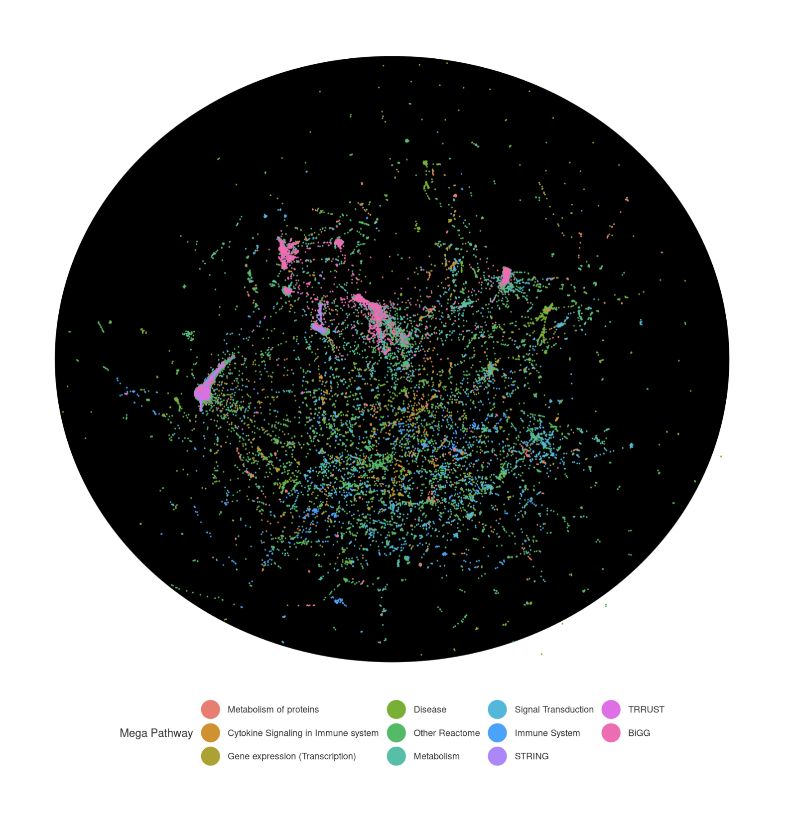
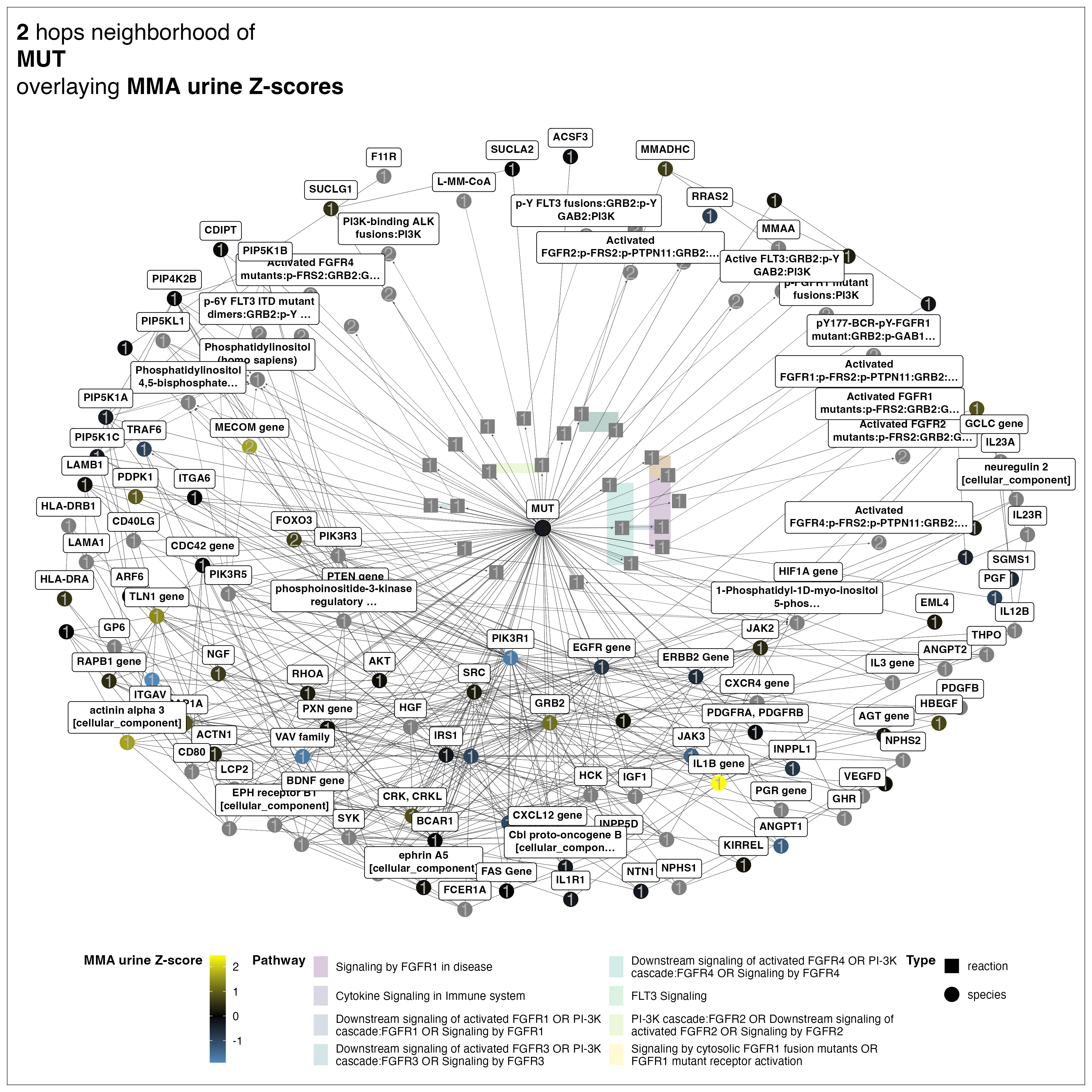
This genome-scale view shows the overall network structure, but I can zoom into any region to examine molecular interactions at high resolution. For example, I can explore the molecular neighborhood of MMUT (labeled as “MUT” in the network) to identify its upstream regulators and downstream targets. This local view reveals how MMUT connects to both regulatory genes (such as AKT and IGF1) and metabolites (like its enzymatic product methylmalonyl-CoA, shown as L-MM-CoA), illustrating the integration of gene regulatory and metabolic networks.

Vertex names may differ from the nomenclature used by individual data sources; however, all merges are based on reliable database identifiers, ensuring accurate molecular relationships. Annotations are organized in Identifiers objects, which track the identifiers across multiple ontologies related to a given entity. These annotations also incorporate SBML’s biological qualifiers, which define relationships such as BQB_IS (identity), BQB_HAS_PART (component of a complex), and BQB_IS_DESCRIBED_BY (reference to supporting literature).

Napistu leverages these annotations both to merge data sources when building the consensus model and to seamlessly integrate high-dimensional datasets with its pathway representations.

I created this visualization — and the subgraph figure you’ll see later — using results from this post. If you’re interested in generating visualizations like this, check out network_visualzation.qmd. Though Napistu is primarily a Python framework, its companion R package, napistu.r, is purpose-built for visualizing Napistu networks. It leverages ggraph for grammar-of-graphics-based visualizations and uses reticulate to bridge R and Python, enabling direct access to Napistu’s data structures and functions.

Adding data to networks

To use an `omics dataset in Napistu, I will:

1. Mount the dataset onto the pathway SBML_dfs, which involves: a. Matching systematic identifiers between the dataset and the pathway to link `omics features with Napistu species. b. Resolving many-to-one mappings (i.e., when multiple features map to the same molecular species). c. Constructing a table indexed by unique species IDs, with dataset variables as columns. d. Adding this table to the species_data attribute of the SBML_dfs. Multiple tables and/or datasets can be stored in species_data.
2. Pass variables to graph vertices a. Use net_create._add_graph_species_attribute to pass variables from one or more species_data tables to a NapistuGraph’s vertices. b. Optionally, variables can be transformed at this stage (e.g., to make them non-negative for personalized PageRank).
3. Use these vertex attributes for downstream analyses, such as setting the reset_proportional_to parameter in personalized PageRank.

Data $\Rightarrow$ SBML_dfs

To identify which results to explore further with network methods, I’ll first review the MuData object from the previous analysis. This summary highlights both MuData-level attributes — such as Multi-Omics Factor Analysis (MOFA) results — and modality-level AnnData attributes, including:

• obs: sample-level metadata
• var: feature-level metadata
• X and layers: measurements
• obsm, varm: tensors defined over samples or features

mdata

MuData object with n_obs × n_vars = 221 × 13922
  uns:  'mofa'
  obsm: 'X_mofa'
  varm: 'LFs'
  2 modalities
    transcriptomics:    221 x 9134
      obs:  'case', 'gender', 'consanguinity', 'mut_category', 'wgs_zygosity', 'acidosis', 'metabolic_acidosis', 'metabolic_ketoacidosis', 'ketosis', 'hyperammonemia', 'abnormal_muscle_tone', 'musc_hypotonia', 'musc_hypertonia', 'fct_respiratory_abnormality', 'dyspnea', 'tachypnea', 'reduced_consciousness', 'lethargy', 'coma', 'seizures', 'general_tonic_clonic_seizure', 'any_GI_problem', 'failure_to_thrive', 'any_delay', 'behavioral_abnormality', 'concurrent_infection', 'urine_ketones', 'dialysis', 'peritoneal_dialysis', 'insulin', 'diet', 'carnitine', 'cobalamin', 'bicarb', 'glucose_IV', 'cobalamin_responsive', 'antibiotic_treatment', 'protein_restriction', 'tube_feeding_day', 'tube_feeding_night', 'tube_feeding_overall', 'language_delay', 'any_neurological_abnormalities_chronic', 'impaired_kidney_fct', 'hemat_abnormality', 'anemia', 'neutropenia', 'skin_abnormalities', 'hearing_impairment', 'osteoporosis', 'failure_to_thrive_chronic', 'global_dev_delay_chr', 'hypotonia_chr', 'basal_ganglia_abnormality_chr', 'failure_to_thrive_or_tube_feeding', 'irritability', 'hyperventilation', 'hypothermia', 'somnolence', 'vomiting', 'dehydration', 'feeding_problem', 'responsive_to_acute_treatment', 'n_passage', 'date_collection', 'date_freezing', 'onset_age', 'OHCblMinus', 'OHCblPlus', 'ratio', 'SimultOHCblMinus', 'SimultOHCblPlus', 'AdoCblMinus', 'AdoCblPlus', 'SimultAdoCblMinus', 'SimultAdoCblPlus', 'prot_mut_level', 'rnaseq_mut_level', 'MMA_urine', 'ammonia_umolL', 'pH', 'base_excess', 'MMA_urine_after_treat', 'carnitine_dose', 'natural_protein_amount', 'total_protein_amount', 'weight_centile_quant', 'length_centile_quant', 'head_circumfernce_quant', 'proteomics_runorder'
      var:  'est_MMA_urine', 'est_OHCblPlus', 'est_case', 'est_responsive_to_acute_treatment', 'p_MMA_urine', 'p_OHCblPlus', 'p_case', 'p_date_freezing', 'p_proteomics_runorder', 'p_responsive_to_acute_treatment', 'log10p_MMA_urine', 'log10p_OHCblPlus', 'log10p_case', 'log10p_responsive_to_acute_treatment', 'q_MMA_urine', 'q_OHCblPlus', 'q_case', 'q_date_freezing', 'q_proteomics_runorder', 'q_responsive_to_acute_treatment', 'stat_MMA_urine', 'stat_OHCblPlus', 'stat_case', 'stat_responsive_to_acute_treatment', 'stderr_MMA_urine', 'stderr_OHCblPlus', 'stderr_case', 'stderr_responsive_to_acute_treatment', 'is_transcriptomics'
      obsm: 'X_pca'
      varm: 'PCs'
      layers:   'log2_centered'
    proteomics: 221 x 4788
      obs:  'case', 'gender', 'consanguinity', 'mut_category', 'wgs_zygosity', 'acidosis', 'metabolic_acidosis', 'metabolic_ketoacidosis', 'ketosis', 'hyperammonemia', 'abnormal_muscle_tone', 'musc_hypotonia', 'musc_hypertonia', 'fct_respiratory_abnormality', 'dyspnea', 'tachypnea', 'reduced_consciousness', 'lethargy', 'coma', 'seizures', 'general_tonic_clonic_seizure', 'any_GI_problem', 'failure_to_thrive', 'any_delay', 'behavioral_abnormality', 'concurrent_infection', 'urine_ketones', 'dialysis', 'peritoneal_dialysis', 'insulin', 'diet', 'carnitine', 'cobalamin', 'bicarb', 'glucose_IV', 'cobalamin_responsive', 'antibiotic_treatment', 'protein_restriction', 'tube_feeding_day', 'tube_feeding_night', 'tube_feeding_overall', 'language_delay', 'any_neurological_abnormalities_chronic', 'impaired_kidney_fct', 'hemat_abnormality', 'anemia', 'neutropenia', 'skin_abnormalities', 'hearing_impairment', 'osteoporosis', 'failure_to_thrive_chronic', 'global_dev_delay_chr', 'hypotonia_chr', 'basal_ganglia_abnormality_chr', 'failure_to_thrive_or_tube_feeding', 'irritability', 'hyperventilation', 'hypothermia', 'somnolence', 'vomiting', 'dehydration', 'feeding_problem', 'responsive_to_acute_treatment', 'n_passage', 'date_collection', 'date_freezing', 'onset_age', 'OHCblMinus', 'OHCblPlus', 'ratio', 'SimultOHCblMinus', 'SimultOHCblPlus', 'AdoCblMinus', 'AdoCblPlus', 'SimultAdoCblMinus', 'SimultAdoCblPlus', 'prot_mut_level', 'rnaseq_mut_level', 'MMA_urine', 'ammonia_umolL', 'pH', 'base_excess', 'MMA_urine_after_treat', 'carnitine_dose', 'natural_protein_amount', 'total_protein_amount', 'weight_centile_quant', 'length_centile_quant', 'head_circumfernce_quant', 'proteomics_runorder'
      var:  'PG.ProteinDescriptions', 'PG.ProteinNames', 'PG.Qvalue', 'est_MMA_urine', 'est_OHCblPlus', 'est_case', 'est_responsive_to_acute_treatment', 'p_MMA_urine', 'p_OHCblPlus', 'p_case', 'p_date_freezing', 'p_proteomics_runorder', 'p_responsive_to_acute_treatment', 'log10p_MMA_urine', 'log10p_OHCblPlus', 'log10p_case', 'log10p_responsive_to_acute_treatment', 'q_MMA_urine', 'q_OHCblPlus', 'q_case', 'q_date_freezing', 'q_proteomics_runorder', 'q_responsive_to_acute_treatment', 'stat_MMA_urine', 'stat_OHCblPlus', 'stat_case', 'stat_responsive_to_acute_treatment', 'stderr_MMA_urine', 'stderr_OHCblPlus', 'stderr_case', 'stderr_responsive_to_acute_treatment', 'is_proteomics'
      obsm: 'X_pca'
      varm: 'PCs'
      layers:   'log2_centered'

Feature-level attributes (e.g., MuData or AnnData’s var, varm, X, or layers) can be seamlessly added to a NapistuGraph using high-level workflows that handle identifier mapping, disambiguation, and complex membership automatically.

Napistu supports three data input types:

• mudata.MuData objects contain multiple AnnData objects where var and varm attributes can be defined across multiple datasets. Results can be stored in separate tables, as separate attributes within the same table, or merged into a single attribute (e.g., combining transcript- and protein-level summaries).
• anndata.AnnData objects contribute systematic identifiers from their var and feature-level summaries come from either the var, varm, X, or layers tables.
• pd.DataFrame objects which include one or more columns with systematic identifiers.

Here, I’ll start with a detailed example using results from a MuData object.

Adding latent factors

In the previous post, I applied Multi-Omics Factor Analysis (MOFA) to decompose the dataset into 30 covarying latent factors. The factor loadings are a 13,900 × 30 matrix: mdata.varm["LFs"].

The prepare_mudata_results_df function prepares this tensor for Napistu by:

• Extracting modality-specific systematic identifiers from var
• Combining them with the corresponding factor loadings
• Returning a dictionary that supports various strategies for merging across modalities

mofa_lfs = prepare_mudata_results_df(
    mdata,
    mudata_ontologies=MUDATA_ONTOLOGIES,
    table_type="varm",
    table_name=FORNY_DEFS.LFS, # this would be autodetected
    results_attrs=LFS_OF_INTEREST,
    table_colnames=[f"LF{i}" for i in range(1, mdata.varm[FORNY_DEFS.LFS].shape[1] + 1)]
)

Below are the first five rows of the MOFA latent factors for each modality:

for modality in MODALITIES:
  
    systematic_id_column = MUDATA_ONTOLOGIES[modality]["index_which_ontology"]
  
    mofa_lfs_examples = (
        mofa_lfs[modality]
        .drop(columns = systematic_id_column)
        .sample(5)
        .copy()
    )
    format_numeric_columns(mofa_lfs_examples, inplace = True)
  
    display_tabulator(
        mofa_lfs_examples,
        caption = f"Extracted latent factors for {modality}",
        column_widths={systematic_id_column : "25%"}
    )

Extracted latent factors for transcriptomics

Extracted latent factors for proteomics

To add these results to an SBML_dfs object, I’ll:

• Create a pandas.DataFrame with 0–1 rows per distinct molecular species in the model
• Store this DataFrame as a key-value pair in the species_data dictionary attribute of the SBML_dfs

Molecular species are linked to various ontologies (e.g., Ensembl, UniProt, Entrez). Napistu can distinguish genes, transcripts, and proteins as distinct molecular species (“dogmatic mode”). However, the loaded model merges these into a single species, ignoring such distinctions.

Merging `omics data into the pathway representation involves:

• Matching based on identifiers
• Resolving collisions (e.g., when transcripts and proteins map to the same species, or multiple proteins map to one molecular species)

These challenges are handled by mount.bind_dict_of_wide_results. In this example, I “stagger” results to keep latent factors separate based on whether they correspond to transcripts or proteins.

mount.bind_dict_of_wide_results(
    sbml_dfs,
    mofa_lfs,
    FORNY_DEFS.MOFA_LFS,
    strategy = "stagger",
    species_identifiers = species_identifiers,
    # ontologies were already renamed to the controlled vocabulary in prepare_mudata_results_df()
    ontologies = None,
    # ignored because species_identifiers is provided
    dogmatic = False,
    # for clarity; default is True
    inplace = True,
    verbose = False
)

The outcome is a single species_data table integrating latent factors from both modalities, mapped onto the model’s molecular species.

example_species_data = sbml_dfs.species_data[FORNY_DEFS.MOFA_LFS].head(5).copy()
format_numeric_columns(example_species_data, inplace = True)
display_tabulator(example_species_data, width="auto", layout="fitDataStretch")

The scverse and matching subpackages are recent additions to Napistu, designed to make the framework more user-friendly. The goal is to reduce technical barriers for researchers by providing streamlined workflows for common formats like MuData and AnnData objects. (Thanks to Vito Zanotelli for encouraging this direction!)

This module was developed using AI-assisted coding, which revealed some interesting insights into the strengths and weaknesses of different AI tools for scientific software development. Language models like Claude were helpful for understanding biological data structures and offering conceptual guidance, but struggled when it came to extending an existing codebase — often suggesting overly complex or impractical solutions. Code-focused AI tools like Cursor proved more effective for the actual implementation work.

The development process followed an iterative approach: first building prototypes to understand the functionality requirements, then drafting comprehensive tests, followed by implementing individual functions with continuous testing, and finally polishing the code with proper documentation and type annotations. This AI-assisted workflow significantly accelerated development while maintaining code quality - a pattern that’s becoming increasingly valuable for scientific software projects.

Adding statistical summaries and modality masks

Having shown how to bind MOFA factor loadings to the pathway, I’ll now add differential expression results.

The disease phenotypes of interest are:

• OHCblPlus: enzymatic activity readout
• MMA_urine: metabolic burden indicator
• case: disease status
• responsive_to_acute_treatment: effectiveness of acute vitamin supplementation

For each phenotype, I’ll add the following statistical summaries:

• estimate: the regression effect size
• statistic: the regression t-statistic
• log10p: the $-\log_{10}(\text{p-value})$ (calculated this way to avoid numerical underflow)
• q-value: the Benjamini-Hochberg FDR-adjusted p-value

I’ll also include the q-values for covariates used in the regressions — namely, the nonlinear associations of freezing_date and proteomics_run_order.

# now we can add .var attributes from the mdata
diffex_results = prepare_mudata_results_df(
    mdata,
    mudata_ontologies=MUDATA_ONTOLOGIES,
    table_type="var",
    results_attrs=VAR_VARS,
    level = "adata"
)

mount.bind_dict_of_wide_results(
    sbml_dfs,
    diffex_results,
    FORNY_DEFS.VAR_LEVEL_RESULTS,
    strategy = "stagger",
    species_identifiers = species_identifiers,
    verbose = False
)

Finally, I’ll add modality-level indicator variables. For loose results in a pandas.DataFrame, I could use bind_wide_results to add them directly to the SBML_dfs.

for modality in MODALITIES:
    anndata_results_df = prepare_anndata_results_df(
        mdata[modality],
        table_type="var",
        index_which_ontology = MUDATA_ONTOLOGIES[modality]["index_which_ontology"],
        results_attrs=ADATA_LEVEL_VARS[modality]
    )

    mount.bind_wide_results(
        sbml_dfs,
        anndata_results_df,
        FORNY_DEFS.MODALITY_VAR_LEVEL_RESULTS_STR.format(modality = modality),
        species_identifiers = species_identifiers,
        ontologies = MUDATA_ONTOLOGIES[modality]["ontologies"]
    )

SBML_dfs $\Rightarrow$ NapistuGraph

Now, I can pass selected attributes from the species_data tables to the NapistuGraph object. While the low-level, flexible set_graph_attrs method (which also supports setting edge attributes) is available, I’ll use the more user-friendly function instead: data_handling.add_results_table_to_graph().

When working with an SBML_dfs loaded from GCS, users can typically rely on the pre-generated NapistuGraph bundled with it. These graphs are:

• Directed (though reversible reactions, such as STRING interactions, appear as paired forward and reverse edges)
• Wired based on a regulatory hierarchy: vertices are arranged in tiers — regulators → catalysts → substrates → reactions → products
• Sensibly weighted: edges reflect meaningful interaction weights where applicable

The only modification I’ll make for this analysis is reversing the graph’s edges, so that signals can flow from effects (e.g., dysregulated genes) upstream to their potential causes (e.g., transcriptional or enzymatic regulators).

Here’s a view of the graph showing a random selection of vertices and edges:

vertex_indices = np.random.choice(len(napistu_graph.vs), 10, replace = False)
vertices_df =(
    pd.DataFrame({
        i : napistu_graph.vs[i].attributes() for i in vertex_indices
    })
    .T
    .assign(sc_Source = ".")
    .set_index("name")
    .fillna(".")
)

edge_indices = np.random.choice(len(napistu_graph.es), 10, replace = False)
edges_df = (
    pd.DataFrame({
        i : napistu_graph.es[i].attributes() for i in edge_indices
    })
    .T
    .assign(sc_Source = ".")
    .set_index(["from", "to"])
)
format_numeric_columns(edges_df, inplace = True)

display_tabulator(vertices_df, caption="Vertices", width="auto", layout="fitDataStretch")
display_tabulator(edges_df, caption="Edges", width="auto", layout="fitDataStretch")

Vertices

Edges

Most NapistuGraph objects — including this one — contain both species and reaction vertices:

• Species vertices represent molecular entities (genes, proteins, metabolites, etc.)
• Reaction vertices represent biochemical or regulatory reactions

This bipartite structure is borrowed from metabolic modeling where metabolites are connected via reaction nodes that define their interconversion. But, the NapistuGraph used here is not a strict bipartite network since species nodes can be connected to other species nodes.

Creating an appropriate graph with data attributes

To prepare the graph for network propagation, I’ll:

1. Reverse all edges to allow signal flow from observed effects to their upstream causes.
2. Add species attributes from species_data to the vertices using add_results_table_to_graph(). This entails specifying which attributes to use and how to transform them to make them suitable for personalized PageRank (non-negative, where larger values represent stronger signals).

# create a copy of the graph
napistu_graph.reverse_edges()
assert napistu_graph.is_reversed

for attr_to_graph in ATTRIBUTES_TO_GRAPH_SPEC:
    
    data_handling.add_results_table_to_graph(
        napistu_graph,
        sbml_dfs,
        attribute_names = attr_to_graph["attribute_names"],
        table_name = attr_to_graph["table_name"],
        transformation = attr_to_graph["transformation"],
        custom_transformations = CUSTOM_TRANSFORMATIONS
    )

Network propagation with Personalized PageRank (PPR)

To link gene-level changes to common regulators, I’ll apply personalized PageRank (PPR) to each vertex attribute in the NapistuGraph. Conceptually, PageRank begins with a signal on a random vertex that, at each step, either:

• Moves to a connected child node with probability $\alpha$
• Resets to a random vertex with probability $1-\alpha$

In PPR, the reset step is biased — rather than resetting to any vertex uniformly, it follows a user-defined probability distribution, often weighted by input signals like gene dysregulation scores. Repeating this random walk causes the signal to accumulate at hub vertices — nodes central to the input signal.

The actual PageRank algorithm finds the stationary distribution of this process using some slick linear algebra - power iteration to find the stationary distribution and sparse matrix storage and operations. This excellent blog post by Stefan Weigert offers a clear and intuitive overview of PPR. For example, here is Stefan’s visualization of a random walk following the PPR process which really nails the intuition for me:

.

Applying PPR

I’ve prepared the conditions for PPR by defining attributes as reset probability distributions (after L1 normalization). To ensure non-negativity and highlight signal strength, I applied ad hoc transformations — like converting $\log_{10}(\text{p-values})$ to $-\log_{10}(\text{p-values})$ and squaring effect sizes. While these choices are reasonable, ideally such transformations would be learned rather than preset.

annotated_vertices = napistu_graph.get_vertex_dataframe()

# find valid attributes - numeric + 1+ non-zero values
invalid_attributes = [x for x in annotated_vertices.columns if annotated_vertices[x].dtype not in ["float64", "int64"] or annotated_vertices[x].nunique() == 1]
valid_attributes = [x for x in annotated_vertices.columns if x not in invalid_attributes]

logger.info(f"Invalid attributes: {invalid_attributes}")
logger.info(f"Valid attributes: {valid_attributes}")

# create masks for each modality
assert [x in valid_attributes for x in REGEXES_TO_MASKS.values()]
valid_attributes = list(set(valid_attributes) - set(REGEXES_TO_MASKS.values()))

ppr_results = net_propagation.net_propagate_attributes(
    napistu_graph,
    attributes = valid_attributes,
    propagation_method = "personalized_pagerank",
    additional_propagation_args = { "damping": 0.85 }
)

Controlling for PPR’s biases

While PPR reveals convergence points of biological signals in a network, it is inherently biased toward highly connected hub nodes — an effect evident when examining vertices with the highest median PPR values across attributes.

top_5_by_median_ppr = (
    ppr_results.median(axis=1)
    .sort_values(ascending=False)[0:5]
    .rename("median PPR")
    .to_frame()
    .merge(
        annotated_vertices[["name", "node_name"]],
        left_index = True,
        right_on = "name"
    )
)
top_5_by_median_ppr["degree"] = napistu_graph.degree(top_5_by_median_ppr.index.tolist())
format_numeric_columns(top_5_by_median_ppr, "{:.2e}", inplace = True)

display_tabulator(top_5_by_median_ppr.reset_index(drop = True), width="500px")

To correct for this, we must address two sources of bias:

1. Topological Bias - Dense network regions with high in-degree nodes tend to attract signals regardless of biological relevance — a common issue in network analysis. Napistu offers several null distributions to address this, the most relevant being:
   • vertex_permutation: A non-parametric method that shuffles signals across vertices.
   • parametric_null: A parametric method that models nulls using a distribution derived from the observed signal. For example, binary data may be modeled with a Bernoulli null distribution.
2. Ascertainment Bias - This bias occurs because experiments measure only a subset of the network. For instance, metabolomics data focus on central carbon metabolism simply because it was measured. To address this, I limited null permutations to resample only from vertices with measured values (e.g., transcriptomics or proteomics nodes identified by modality masks).

Building null distributions

To robustly assess signal enrichment, I generated 500 null PPR distributions by shuffling reset probabilities among measured vertices (using modality masks). Each vertex’s observed PPR value was compared to its null distribution, allowing its empirical quantile to serve as a non-parametric p-value.

Because biological signals can both enrich and deplete regions, I separately characterized signals in the right (enrichment) and left (depletion) tails by:

• Computing two-tailed p-values where either strong enrichment or depletion would result in a small p-value
• Assigning features as enriched or depleted based on their quantile (greater than or less than 0.5)
• Applying FDR correction separately to enriched and depleted sets

attr_masks = dict()
for attr in valid_attributes:
    for regex, mask in REGEXES_TO_MASKS.items():
        if re.search(regex, attr):
            attr_masks[attr] = mask
            continue

    if attr not in attr_masks:
        logger.info(f"Could not find a modality-specific mask for {attr}; using {attr} as its own mask")
        # default behavior is to use the attribute as its own mask but adding it anyways to be explicit
        attr_masks[attr] = attr
        
if os.path.isfile(PPR_NULL_TMP_PATH) and not OVERWRITE:
    logger.info(f"Loading PPR nulls from cache at {PPR_NULL_TMP_PATH}")
    ppr_with_nulls = pd.read_csv(PPR_NULL_TMP_PATH, sep="\t", index_col=0)
else:
    logger.info(f"Calibrating PPR enrichments by permuting vertex attributes among masked vertices")
    ppr_with_nulls = net_propagation.network_propagation_with_null(
        napistu_graph,
        attributes = valid_attributes,
        mask = attr_masks,
        propagation_method = "personalized_pagerank",
        additional_propagation_args = { "damping": 0.85 },
        null_strategy = "vertex_permutation",
        n_samples = N_NULL_SAMPLES,
        verbose = True    
    )   

    logger.info(f"Saving PPR nulls to cache at {PPR_NULL_TMP_PATH}")
    ppr_with_nulls.to_csv(PPR_NULL_TMP_PATH, sep="\t")

Comparing subgraph enrichments and depletions

Next, I will calculate p-values and q-values stratified by attribute and distinguishing enrichments and depletions.

# name index to vertex_id
tall_ppr_enrichments = (
    ppr_with_nulls
    .reset_index()
    .rename(columns={"index": "vertex_name"})
    .melt(id_vars=["vertex_name"], var_name="attribute", value_name="ppr_null_quantile")
    .assign(p_value = lambda x: hypothesis_testing.quantile_to_pvalue(x["ppr_null_quantile"], "two-tailed"))
    .assign(is_enriched = lambda x: x["ppr_null_quantile"] > 0.5)
    # correct for 0 p-values by flooring based on the # of null samples
    .assign(p_value = lambda x: floor_pvalue_by_resolution(x["p_value"], N_NULL_SAMPLES))
    .assign(nulls_gt_observed = lambda x: ((1 - x["ppr_null_quantile"])*N_NULL_SAMPLES).fillna(-1).astype(int))
)

# combine observed and null summaries
tall_ppr_results =  (
    ppr_results
    .reset_index()
    .rename(columns={"index": "vertex_name"})
    .melt(id_vars=["vertex_name"], var_name="attribute", value_name="ppr_score")
    .merge(tall_ppr_enrichments, on=["vertex_name", "attribute"])
    .dropna(subset=["p_value"])
)

fdr_controlled_results = multi_model_fitting.control_fdr(
    tall_ppr_results,
    grouping_vars = ["attribute", "is_enriched"],
    require_groups = True
)

Now, we can compare the distributions of enrichment and depletion p-values aggregating over all attributes.

plot_ppr_enrichment_histograms(fdr_controlled_results)

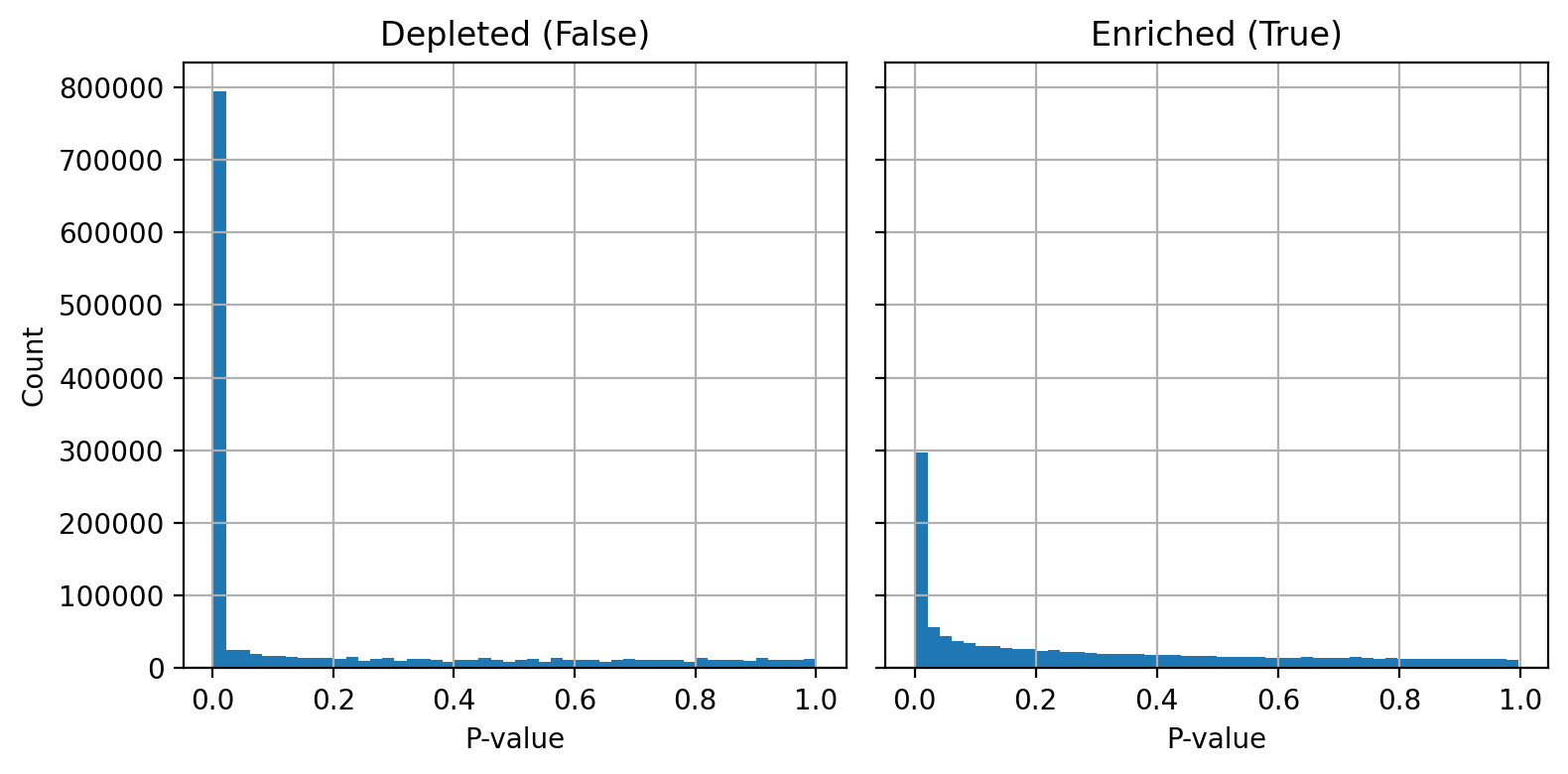
From these p-value histograms I can see that there are vertices which are enriched and depleted for my signals and the depletions are particularly pronounced. This observation is why I stratified enrichments and depletions when calculating FDR.

Identifying enriched subgraphs

To explore the subnetworks enriched for each attribute, I will filter the data to include only vertices significantly enriched for a given attribute (q < 0.1). I will then count the number of enriched vertices for each attribute:

n_enriched_vertices = fdr_controlled_results.query("is_enriched == True").query("q_value < 0.1").value_counts("attribute")

# add back zeros
missing_attributes = set(fdr_controlled_results["attribute"].unique()) - set(n_enriched_vertices.index.tolist())
missing_attributes

n_enriched_vertices = (
    pd.concat([
        n_enriched_vertices,
        pd.Series({attr: 0 for attr in missing_attributes}).rename("count")
    ])
)

# reformat the attributes to include modality and measure
attr_metadata = dict()
for key in n_enriched_vertices.index.tolist():
    for mod in MODALITIES:
        # match str
        if re.search(mod, key):
            attr_metadata[key] = {
                "modality" : mod,
                "variable" : re.sub(f"_{mod}$", "", key)
            }
            break

    if key not in attr_metadata:
        attr_metadata[key] = {
            "modality" : "unknown",
            "variable" : key
        }

attr_metadata_df = (
    pd.DataFrame(attr_metadata).T
    .merge(VAR_METADATA, on = "variable", how = "left")
).assign(attribute=lambda x: x.apply(lambda row: f"{row['variable']}_{row['modality']}", axis=1)).set_index("attribute")

attr_signif_counts = pd.concat(
    [
        n_enriched_vertices,
        attr_metadata_df
    ],
    axis = 1
)

fig, ax = create_stacked_barplot_seaborn(attr_signif_counts)

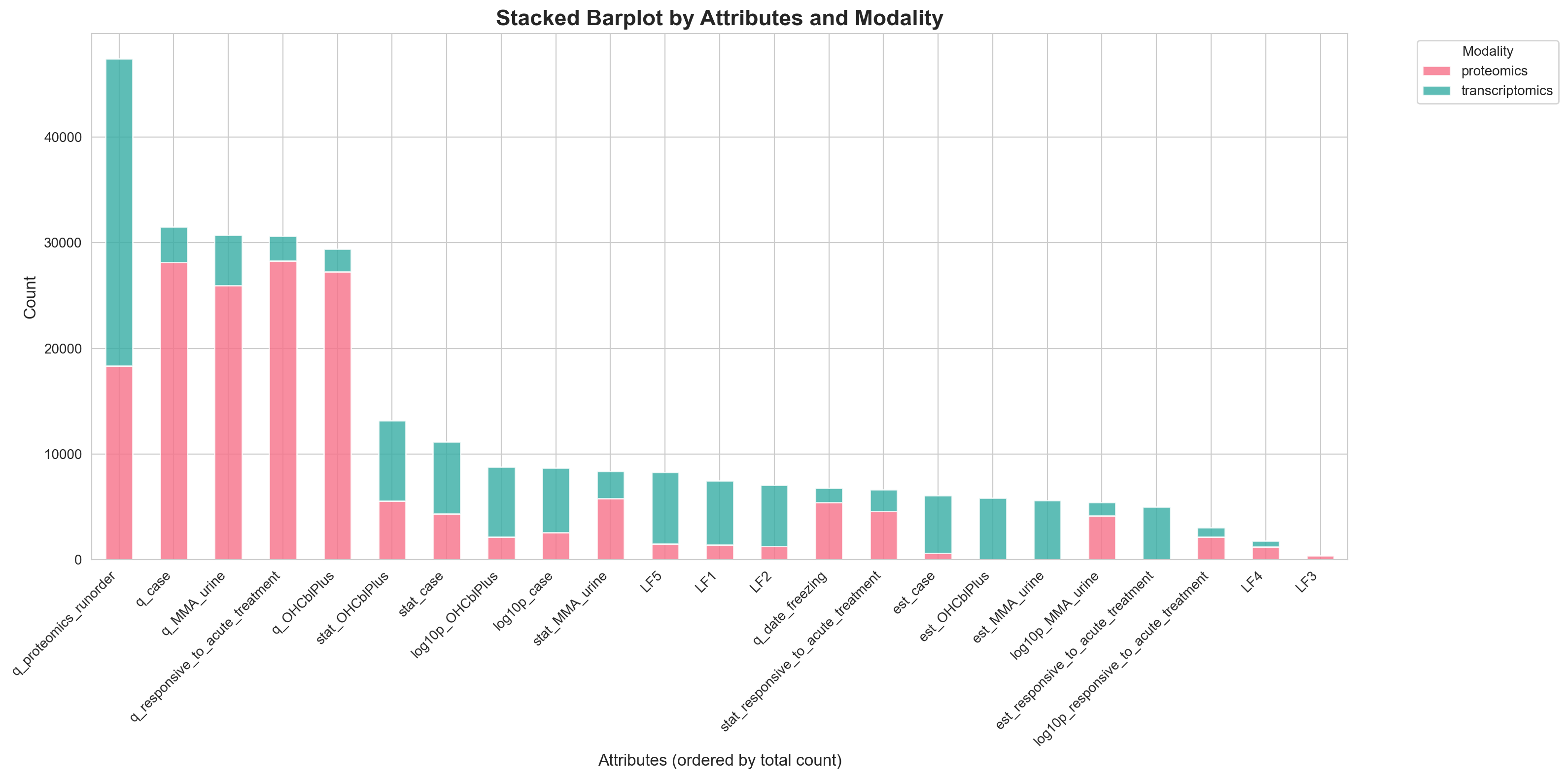
This plot shows that setting vertex reset probabilities based on $-\log_{10}(\text{q-values})$) produces the largest subgraph of upstream enriched vertices. A similar result was observed with a hard thresholding approach, where vertices with q > 0.1 were assigned a reset probability of 0. Notably, despite being monotonic transformations, $-\log_{10}(\text{q-values})$ diverge substantially from $-\log_{10}(\text{p-values})$.

So, which metric is more trustworthy? I lean toward p-values — if everything becomes significant, it’s as uninformative as if nothing is significant. The strong enrichment for proteomics run order in the transcriptomics data, despite minimal nominal significance, is a red flag that q-values may be inappropriate in this context.

Choosing appropriate transformations for network propagation underscores a fundamental challenge in biological network analysis: the lack of clear benchmarks. Unlike many machine learning domains, we often lack ground truth, making it difficult to select hyperparameters or validate methodological choices systematically.

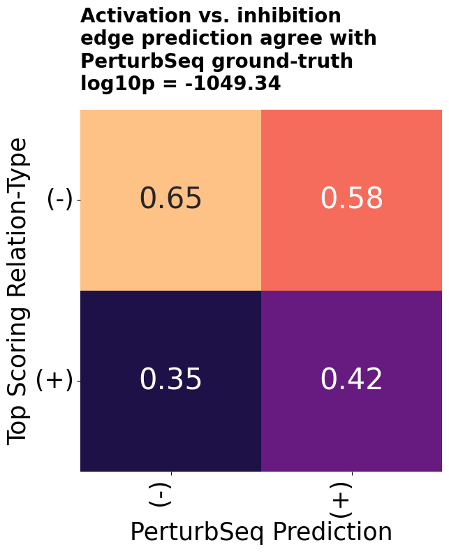
Supervised machine learning offers a path forward by reframing ambiguous biological questions as well-defined prediction tasks, yielding two key advantages. First, machine learning methods can potentially capture functional relationships more accurately than algorithms like personalized PageRank — provided the training data and prediction tasks reflect meaningful biological objectives. The increasing availability of Perturb-seq data, for example, enables direct prediction of regulatory relationships from expression signatures. Second, even when using traditional network methods, supervised tasks can inform hyperparameter tuning and network design in contexts where ground truth is scarce.

For example, if a network representation accurately recovers masked protein–protein interactions, it suggests that the underlying data integration and edge-weighting strategies capture meaningful biology. These insights can then refine traditional network analyses, such as the personalized PageRank approach used here. This creates a virtuous cycle in which machine learning tasks guide the construction of better networks, which in turn enhance the effectiveness of both ML and non-ML methods for biological discovery.

Interpreting network enrichments

To summarize the strongest network-based enrichments, I took the union of the top five enriched vertices per attribute and measured how often their enrichment signal exceeded the null across 500 permutations. (This is akin to comparing the rank of a top signal for one attribute against its ranks across others. However, because the coarse-grained empirical nulls create many tied ranks — causing abrupt jumps from 1 to hundreds or thousands — the raw ranks are difficult to interpret.)

ppr_signif_w_metadata = (
    fdr_controlled_results
    .merge(attr_metadata_df, on = "attribute", how = "left")
    # remove q-value based ranking
    .query('summary != "q"')
    # sort each attribute in ascending order by q-value and provide the rank, handling ties appropriately
    .assign(rank = lambda x: x.groupby(["attribute", "is_enriched"])["q_value"].rank(method="min", ascending=True))
    # replace rank with . if q-value is above 0.1
    .assign(rank = lambda x: x["rank"].where((x["q_value"] <= 0.1) & (x["is_enriched"] == True), "."))
    # similar approach but work with quantiles relative to null
    .assign(display_nulls_gt_observed = lambda x: x["nulls_gt_observed"].where((x["q_value"] <= 0.1) & (x["is_enriched"] == True), "."))
)

# loop through
phenotypes_of_interest = PPR_LINEAR_PHENOTYPES
for phenotype in phenotypes_of_interest:

    phenotype_ppr_results = ppr_signif_w_metadata.loc[ppr_signif_w_metadata["phenotype"] == phenotype]

    # find top N vertices for each attribute 
    top_phenotype_vertices = phenotype_ppr_results.query("q_value < 0.1 & is_enriched == True").sort_values(["q_value", "ppr_score"], ascending = [True, False]).groupby("attribute").head(5)["vertex_name"].unique()

    top_phenotype_stats = phenotype_pivot = (
        phenotype_ppr_results.query("vertex_name in @top_phenotype_vertices").merge(
            annotated_vertices[["name", "node_name", "node_type"]],
            left_on = "vertex_name",
            right_on = "name"
        )
        #.assign(rank=lambda x: x["rank"].apply(lambda val: str(int(float(val))) if val != "." else val))
        #.pivot_table(index = ["modality", "summary"], columns = "node_name", values = "rank", aggfunc="first")
        .pivot_table(index = ["modality", "summary"], columns = "node_name", values = "display_nulls_gt_observed", aggfunc="first")
        .T
    )

    # Apply to your table
    reordered_table = (
        reorder_by_rank_sum(top_phenotype_stats)
        .fillna(".")
    )

    display_tabulator(
        reordered_table,
        caption=f"Association ranks for {phenotype}",
        wrap_columns=["node_name"],
        column_widths={"node_name" : "50%"}
    )
    
    display(HTML('<div style="margin-bottom: 30px;"></div>'))

Association ranks for MMA_urine

Association ranks for case

Association ranks for OHCblPlus

Association ranks for responsive_to_acute_treatment

These results are fascinating:

• MUT, the major genetic cause of MMA, frequently appears.
• Both MUT’s substrate, methylmalonyl CoA (L-MM-CoA), and its product, succinyl CoA (SUCC-CoA), are represented along with a number of other metabolites discussed in the original study such as glutamine. Recovering metabolite associations is particularly interesting because there was no metabolomics data on these cell lines.
• 2-oxoglutarate (2OG), aka alpha-ketoglutarate, appears in several subgraphs. It is the natural counterpart to dimethyl-oxoglutarate, which Forny et al., demonstrated can rescue the MMA-associated metabolic defect.

Transcriptomics associations frequently highlight growth-related genes (e.g., cyclins, IGF1, EGF/R), suggesting that cell line growth rate may be confounded with disease severity. This underscores the inherent biological variability in these datasets. Ideally, doubling time should be included as a covariate in future analyses.

Visualizing induced subgraphs

To more comprehensively visualize these enriched vertices, I generated induced subgraphs retaining both enriched vertices and their molecular interactions. Below is an example focused on MMA urine proteomics:

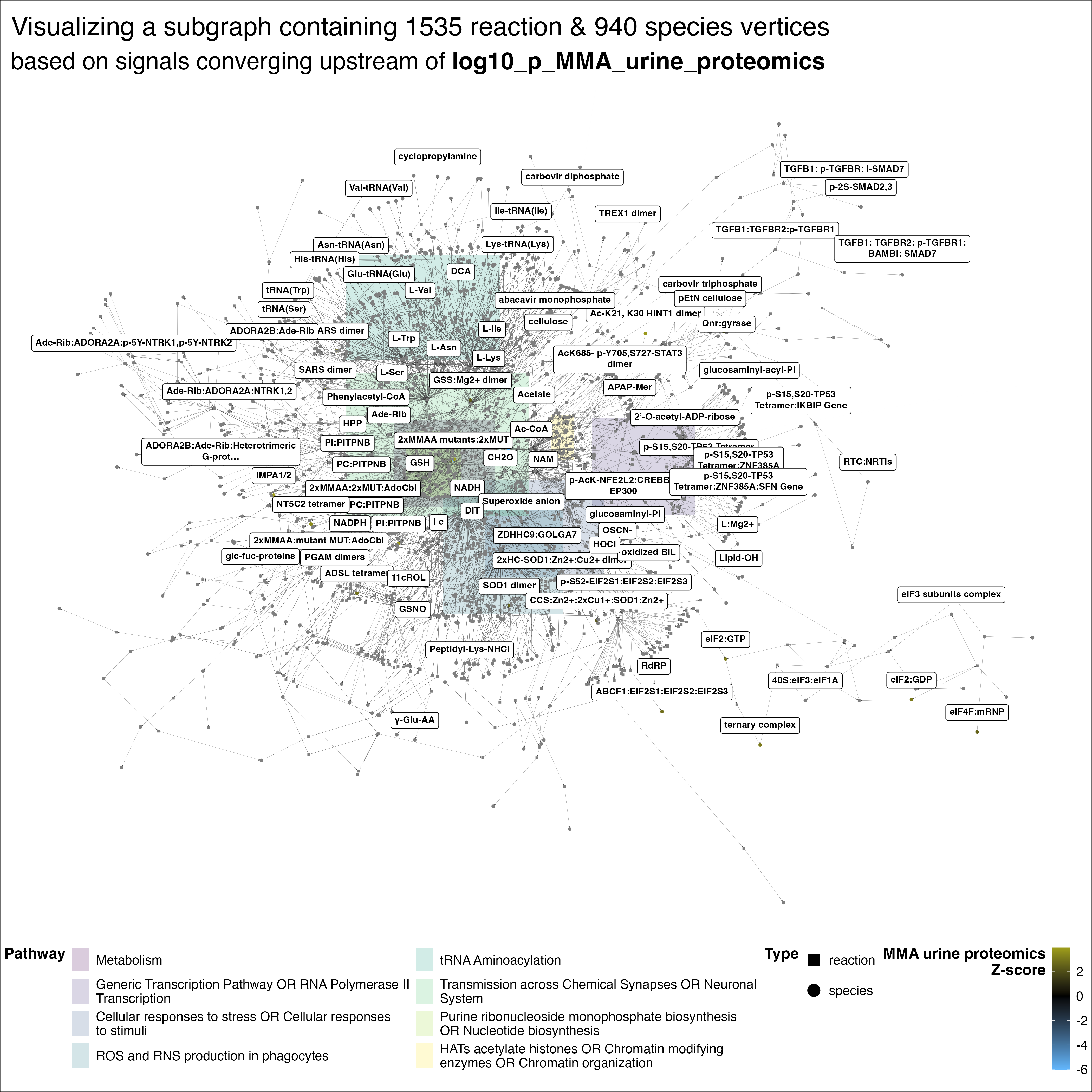
This plot spans the enzymatic causes of MMA — deficiencies in propionate metabolism — with related metabolic effects, such as altered glutamine and glutamate levels, previously observed in MMA patients. Beyond these reassuring associations, the analyses also implicate additional regulatory pathways, including sirtuins and ROS signaling. To investigate any of these regulators, the graph can be traversed to generate causal, mechanistic hypotheses linking upstream regulators to downstream molecular effects.

We know far more about how proteins shape metabolism than how metabolism influences proteins and gene expression. Against this backdrop, it’s notable that sirtuins and ROS signaling emerged — two of the more well-characterized pathways involved in metabolic sensing. Sirtuins function as metabolic sensors by using NAD+ as a cofactor for their histone deacetylase activity, directly linking cellular energy status to chromatin remodeling and the transcriptional regulation of metabolic genes. Reactive oxygen species act as secondary messengers, modulating transcription factor activity and epigenetic modifications to translate metabolic stress and mitochondrial dysfunction into adaptive gene expression programs.

Nonetheless, the hub-like roles of NADH and other cofactors make them challenging to interpret mechanistically. Take water as an example; though not a cofactor, water frequently participates in reactions, many of which produce or consume it. However, the flux of water in individual reactions is negligible compared to its large pool size, so it’s rarely considered a regulated entity or regulator. To address this issue, water is removed from all reactions during the drop_cofactors step of the pathway build process. While this violates mass balance, it preserves the regulatory intent of the SBML_dfs and NapistuGraph.

Handling NADH is more nuanced. In the drop_cofactors step, NAD+ and NADH are removed from reactions only when both are present and NADH acts as the substrate. The rationale is that many reactions consume small amounts of energy (NADH → NAD+) without significantly affecting cellular energetics, whereas energy production (NAD+ → NADH) is typically more physiologically meaningful.

Summary and next steps

This analysis demonstrates how personalized PageRank on genome-scale networks can transform statistical associations into mechanistic biological insights. This approach:

• ✅ Recovered known regulators (e.g., MMUT)
• ✅ Validated and expanded findings on glutamine/glutamate metabolism
• ✅ Linked statistical results to coherent subgraphs of molecular interactions
• ✅ Identified new regulatory hypotheses (e.g., sirtuins, ROS signaling)

By tracing disease signals upstream, we uncover coordinated regulatory modules driving MMA pathophysiology — insights that would be difficult to glean from gene lists alone.

What Napistu provides

Napistu is a comprehensive genome-scale network biology framework designed to bridge the gap between pathway databases and practical analysis. It integrates diverse biological data sources — such as Reactome, BiGG, TRRUST, STRING — into unified network representations that capture both metabolic and gene-centered regulatory mechanisms. It addresses many of the complex data engineering challenges which emerge when working with pathway data including identifier mapping, information consolidation, and translating biological pathways into analysis-ready graph structures

This allows researchers to focus on biological discovery rather than data munging.

Methodology takeaways

This post outlines a workflow for integrating multimodal genomics data with genome-scale biological networks by:

• Extracting feature-level data from AnnData or MuData objects from the scverse project and adding them to a Napistu pathway representation
• Transforming pathway-associated data into vertex attributes on a genome-scale molecular network
• Aggregating signals using network propagation to identify subgraphs enriched for biological signals.

A critical challenge addressed here is that network propagation methods, like personalized PageRank, naturally concentrate signal in hub nodes. This bias arises from two sources:

• Topological bias (due to network structure), and
• Ascertainment bias (due to limited experimental coverage).

To overcome this, I created modality-specific vertex permutation null distributions, allowing me to distinguish genuine biological enrichments from connectivity artifacts.

Napistu’s disease-agnostic design supports any dataset with systematic molecular identifiers. Its modular architecture allows researchers to swap pathway sources, topologies, or propagation algorithms, making it highly adaptable across diverse biological applications.

Try it yourself!

The Napistu framework and all associated analysis workflows are open source and ready to use. The human consensus network featured here is available for direct download from my public repository, and the well-documented code serves as a robust template for applying these methods to your own data.

Whether you’re investigating rare diseases, cancer, or complex traits, Napistu provides a systematic pipeline that transforms statistical associations into mechanistic insights.

🔗 Get started: github.com/napistu/napistu