Timecourses are a powerful experimental design for evaluating the impact of a perturbation. These perturbations are usually chemicals because chemicals, such as a drug, can be introduced quickly and with high temporal precision. Although, with some technologies, such as the estradiol-driven promoters that I used in the induction dynamics expression atlas (IDEA), it is possible to rapidly perturb a single gene further increasing specificity and broadening applicability. By rapidly perturbing individuals, they can be synchronized based on the time when dosing began. We often call this point when dosing begins “time zero” while all subsequent measurements correspond to the time post perturbation. (Since time zero corresponds to a point when a perturbation is applied, but will not yet impact the system, this measurement is usually taken before adding the perturbation.)
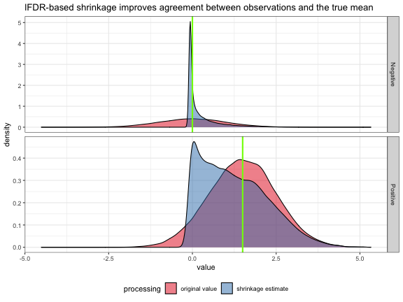
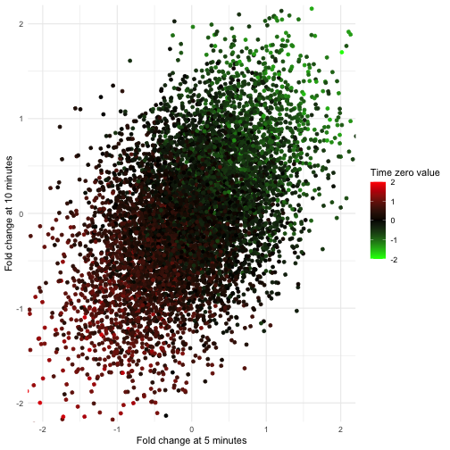
One of the benefits of collecting a time zero measurement is it allows us to remove, or account for, effects that are shared among all time points. In many cases this may just amount to analyzing fold-changes of post-perturbation measurement with respect to their time zero observation, rather than the original measurements themselves. This can be useful if there is considerable variation among timecourses irrespective of the perturbation, such as if we were studying humans or mice. Similarly, undesirable variation due to day-to-day variation in instruments, sample stability, or any of the many other factors which could produce batch effects, can sometimes by addressed by measuring each timecourse together and working with fold-changes. In either case, correcting for individual effects using pre-perturbation measurements will increase our power to detect perturbations’ effects.
Aside from correcting for unwanted variation, the kinetics of timecourses are a rich source of information which can be either a blessing or a curse. With temporal information, ephemeral responses can be observed. We can see both which features are changing and when they are changing. And, the ordering of events can point us towards causality. In practice, each of these goals can be difficult, or impossible to achieve, leaving us with a nagging feeling that we’re leaving information on the table. There are many competing options for identifying differences in timecourses, few ways of summarizing dynamics in an intuitive way, and causal inference is often out of reach. In this post, and others to follow, I’ll pick apart a few of these limitations, discussing developments that were applied to the IDEA, but will likely be useful for others thinking about biological timeseries analysis (or other timeseries if you are so inclined!). Here, I evaluate a few established methods for identifying features which vary across time and then introduce an alternative approach based on the Multivariate Gaussian distribution and Mahalanobis distance which increases power and does not require any assumptions about responses’ kinetics.