Distinguishing Activation from Inhibition with Relation-Aware Graph Neural Networks

In my last post, I discussed self-supervised edge prediction as a way of embedding genes using a gene-regulatory network.

This approach allows genes, metabolites, drugs and other vertices to be connected based on shared network topology. However, to date I’ve only discussed edge prediction using a dot-product head, where a vertex-pair’s edge support is a direct readout of their similarity in embedding space (𝐚 · 𝐛). While surprisingly powerful, this head has limitations when vertices are heterogeneous or interact in qualitatively different ways — particularly when we want to distinguish between activation and inhibition.

Here, I explore more expressive approaches for learning mappings between A → B by evaluating both general edge prediction heads (like MLPs) and “relation-aware” heads that can learn distinct mappings for different edge types. The post will cover:

• Data model and training changes enabling relation-specific predictions
• Geometric analysis revealing how relation-aware heads encode regulatory semantics
• PerturbSeq validation demonstrating successful prediction of signed regulatory interactions
• Pre-trained models available on HuggingFace

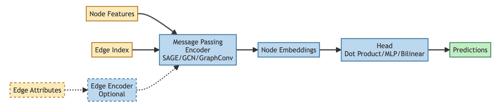
Edge prediction is a powerful approach for predicting regulatory relationships between molecular species, but not all regulatory relations are equivalent. They vary both in how molecules interact (physically, functionally, mechanistically) and in the consequences of these interactions (activation, inhibition, ambiguous effects, or no effect). While the edge encoder partially captures this information to weight message passing, the ultimate prediction is a single continuous score representing edge likelihood — without distinguishing the type of interaction.

Ideally, I want models that can predict not just whether an interaction occurs, but how it occurs. This led me to relation-aware approaches. Relations are commonly discussed in the context of knowledge graphs, where qualitatively different vertex types are connected by different relationship types. For example, embedding the Open Targets knowledge graph organizes genes and phenotypes in a common manifold while also connecting drugs, chemical probes, and other entity types. Learning relation-aware edges defines specific transformations that map between distinct regions of the embedding space.

However, I will be focusing on learning relation-types within a largely homogeneous vertex set — primarily genes and metabolites that can serve multiple regulatory roles. This presents a greater challenge for relation-aware methods, as vertices cannot be cleanly separated by type, and the same molecule may act as both activator and inhibitor in different contexts.

Workflow updates supporting relation prediction

Building robust relation-aware models required improvements to both the Napistu-Torch training framework and the underlying data model.

General framework improvements:

• Hugging Face integration for reproducible datasets and sharing pre-trained models
• Training enhancements including Weights & Biases sweep support and resumable training
• Transfer learning capabilities for loading pre-trained encoders and fine-tuning models

Relation-specific data model changes:

• Reaction vertex removal to enable direct edge prediction between molecular species
• Relation-type labels derived from source and target Systems Biology Ontology (SBO) role annotations

Restructuring the NapistuGraph - no more reaction vertices

Earlier versions of Napistu included both molecular species (proteins, metabolites, drugs, etc.) and reaction vertices. For complex regulatory mechanisms like enzymatic reactions, this provided a clear functional description anchoring pairwise molecular interactions. This was also useful for network visualization, since reactions from common sources — particularly the many narrowly-scoped Reactome pathways — provide ideal labels for network neighborhoods.

However, including reactions has a major downside — individual edges lose their meaning. For example, an enzyme transforming A → B would be encoded as two separate edges (A → R, and R → B). For many purposes this is fine, but for edge prediction it adds more noise than signal. For the model to learn what an A → R → B reaction represents, it would need to encode B’s embedding within the R embedding. This is both computationally difficult and conceptually unnecessary, so for GNNs I’m moving to direct A → B connections.

Predicting direct connections introduces a wrinkle; I had previously enforced that no more than one edge could connect an A-B pair. Moving to a reaction-less graph, I relaxed this constraint so multiple edges can now connect the same vertex pair. This allows activating, inhibitory, and interaction edges to simultaneously exist — relationships that would have previously been distinguished by their intermediate reaction vertices.

Adding relation_type to NapistuData

When constructing the network graph, I encode each mechanism as a series of pairwise interactions, with each participant assigned a role from the SBO controlled vocabulary. SBO terms — like interactor, stimulator, inhibitor, modifier, and modified — capture the distinct ways molecules participate in regulatory mechanisms. To create relation_type labels for edges, I constructed composite labels by combining each edge’s source and target SBO terms, such as “catalyst → reactant,” “interactor → interactor,” and “stimulator → modified.”

NapistuData (a subclass of PyG’s Data), supports relations through two optional attributes: relation_type and its associated relation_manager (for tracking label metadata). Creating these relation types is elegantly handled as an extension of the existing “edge strata” functionality, which organizes edges based on vertex and/or species type to create hard negative samples.

Fitting relation-(un)aware models

During standard edge prediction, we score a possible edge based on the source and target vertices’ embeddings. For relation prediction, we additionally provide heads with a relation_type integer to distinguish different types of relations. To evaluate different head architectures, I trained a range of relation-aware heads alongside simpler relation-unaware baselines.

To enable fair and efficient comparison across heads, I first trained a 128-dimensional GraphConv message passing encoder with a 32-dimensional edge encoder and a simple dot-product head. I deployed this pre-trained model to Hugging Face, then initialized each head of interest with the pre-trained encoder weights.

To leverage this pretraining, I made three key changes to the training regime:

• Lowered the learning rate substantially from 0.003 (original dot-product head) to 0.0005 (transfer learning experiments)
• Used the one-cycle scheduler to gradually ramp up the learning rate
• Initialized expressive heads with init_as_identity settings (when appropriate) so they started from a similar state as the pre-trained dot-product head

To address the imbalanced distribution of relation types in the training data, I applied relation-weighting to each head’s loss function (binary cross-entropy for most heads and a margin-based loss for TransE and RotatE). Each relation type’s loss contribution is weighted by 1/√(relation-type count), down-weighting abundant relation types (like “interactor → interactor”) while emphasizing rare but biologically important ones (like “inhibitor → modified”). This ensures that the models learn to predict all relation types effectively, rather than primarily optimizing for the most common edges.

I fitted all models using model-specific configs and the Napistu-Torch CLI.

Reproducing this analysis

This analysis is fully reproducible — all code, data, and model configurations are provided so you can run the complete workflow on your own machine.

Environment setup:

1. Install uv (or use pip if preferred).

2. Set up a Python environment:

uv venv --python 3.11
source .venv/bin/activate
# Core dependencies
uv pip install torch==2.8.0
uv pip install torch-scatter torch-sparse -f https://data.pyg.org/whl/torch-2.8.0+cpu.html
uv pip install napistu==0.8.5
# pin wandb to 0.22.x for compatibility
uv pip install wandb==0.22.3 
uv pip install "napistu-torch[pyg,lightning,analysis]==0.3.6"
# For rendering the notebook
uv pip install ipykernel nbformat nbclient
python -m ipykernel install --user --name=blog-staging

1. Download the relation_prediction.qmd notebook (or copy relevant code blocks).

2. Choose your path:

   • Using pre-trained models (recommended): The notebook will load the models from Hugging Face on-the-fly.
   • Training from scratch: Download the model configs and training shell script to train models yourself.

3. Configure WORKING_DIR in the following code block to point to your working directory.

Configuration and imports

# standard library imports
from itertools import combinations
import os
from pathlib import Path
import textwrap

# 3rd party imports
from torch import abs
import torch.nn.functional as F
from matplotlib import pyplot as plt
from napistu.ingestion.perturbseq import (
    assign_predicted_direction,
    load_harmonizome_perturbseq_datasets,
    _get_distinct_harmonizome_perturbseq_interactions,
)
from napistu.ingestion.constants import (
    SIGNED_PERTURBATION_TYPES,
    STRONG_ORDERED_SIGNED_PERTURBSEQ_DIRECTIONS,
)
import napistu.utils as napistu_utils
import numpy as np
import pandas as pd

# import a couple of functions used by just the posted version of the blog
# pip install git+https://github.com/shackett/shackett-utils.git
from shackett_utils.utils import pd_utils
from shackett_utils.blog.html_utils import display_tabulator

# napistu-torch imports
from napistu_torch.evaluation.manager import RemoteEvaluationManager
from napistu_torch.visualization.basic_metrics import plot_auc_only, _extract_metric
from napistu_torch.visualization.advanced_metrics import plot_combined_grouped_barplot
from napistu_torch.evaluation.relation_prediction import (
    calculate_relation_type_confusion_and_correlation,
    compare_relation_type_predictions_to_perturbseq_truth,
    get_perturbseq_edgelist_tensor,
    summarize_relation_type_aucs,
)
from napistu_torch.models.constants import HEAD_DESCRIPTIONS
from napistu_torch.utils.tensor_utils import (
    compute_correlation_matrix,
    compute_effective_dimensionality,
    compute_spearman_correlation_torch,
)
from napistu_torch.visualization.heatmaps import plot_heatmap

WORKING_DIR = Path(os.path.expanduser("~/Desktop/relation_prediction_experiments"))
PATH_TO_NAPISTU_STORE = WORKING_DIR / ".store"

MODEL_DISPLAY_ORDER = [
    "dot_product",
    "mlp",
    "attention",
    "distmult",
    "rotate",
    "transe",
    "relation_attention",
    "relation_gated_mlp",
    "relation_attention_mlp",
]

MODEL_HF_REPOSITORIES : dict[str, tuple[str, str]] = {
    "dot_product" : ("seanhacks/relation_prediction_dotprod_128e", "20251229"),
    "mlp" : ("seanhacks/relation_prediction_mlp_128e", "20251229"),
    "attention" : ("seanhacks/relation_prediction_attention_128e", "20251229"),
    "distmult" : ("seanhacks/relation_prediction_distmult_128e", "20251229"),
    "rotate" : ("seanhacks/relation_prediction_rotate_128e", "20251229"),
    "transe" : ("seanhacks/relation_prediction_transe_128e", "20251229"),
    "relation_attention" : ("seanhacks/relation_prediction_relationattention_128e", "20251229-2"),
    "relation_gated_mlp" : ("seanhacks/relation_prediction_relationgatedmlp_128e", "20251229"),
    "relation_attention_mlp" : ("seanhacks/relation_prediction_relationattnmlp_128e", "20251229"),
}

RELATION_AWARE_FOCUSED_HEADS = [
    "distmult",
    "transe",
    "relation_gated_mlp",
    "relation_attention_mlp"
]

PERTURBSEQ_RELATION_TYPES = ["inhibitor -> modified", "stimulator -> modified"]

# local caches
LOCAL_HARMONIZOME_DATA_DIR = "/tmp/harmonizome_data"
CROSS_RELATION_PREDICTION_CACHE = "/tmp/cross_relation_prediction_matrices.pkl"

Comparing relation-(un)aware models

To compare the trained models, I will load their checkpoints and evaluation metrics using Napistu-Torch’s RemoteEvaluationManager, which provides a unified interface for accessing model weights, training configs, and Weights & Biases summaries directly from Hugging Face. (If you are working with local models, you can instead use the similar LocalEvaluationManager, which directly interacts with Weights & Biases and local models and data.)

eval_managers = dict()
for model_name, model_info in MODEL_HF_REPOSITORIES.items():
    model_repo, model_version = model_info
    eval_managers[model_name] = RemoteEvaluationManager.from_huggingface(
        model_repo,
        data_store_dir = PATH_TO_NAPISTU_STORE,
        revision = model_version,
    )

# for local evaluation, instead do this:
# from napistu_torch.evaluation.manager import LocalEvaluationManager
# EXPERIMENT
# eval_managers = dict()
# for experiment in MODEL_DISPLAY_ORDER:
#     experiment_path = <<PATH_TO_EXPERIMENT_DIR>>
#     eval_managers[experiment] = LocalEvaluationManager(experiment_path)

# Load pre-calculated WandB summaries directly from HuggingFace
run_summaries = {exp: manager.get_run_summary() for exp, manager in eval_managers.items()}

# Load all of the trained models
models = {k : v.load_model_from_checkpoint() for k, v in eval_managers.items()}

# Count trainable parameters in each head
n_head_params = {k : sum(p.numel() for p in v.task.head.head.parameters()) for k, v in models.items()}

# connect to the NapistuDataStore and load the NapistuData instance which all models were trained on
# all of the experiments have the same value so we just need to pick an arbitrary one

napistu_data_store = eval_managers["distmult"].napistu_data_store
napistu_data = napistu_data_store.load_napistu_data("relation_prediction")
relation_types = list(napistu_data.relation_manager.label_names.values())
species_identifiers = napistu_data_store.load_pandas_df("species_identifiers")
name_to_sid_map = napistu_data_store.load_pandas_df("name_to_sid_map").reset_index()
name_to_sid_map["integer_id"] = range(len(name_to_sid_map))

if not all(name_to_sid_map["name"] == napistu_data.ng_vertex_names):
    raise ValueError("name_to_sid_map does not match napistu_data.ng_vertex_names")

Model architecture overview

I evaluated seven different head architectures spanning three categories:

• Edge prediction (relation-unaware): Simple heads that predict edge existence without distinguishing relation types. These serve as baselines to assess whether relation-aware methods provide meaningful improvements.
• Knowledge graph embedding: Methods originally developed for heterogeneous knowledge graphs (like TransE and DistMult) that learn relation-specific transformations.
• Relation prediction (expressive heads): Custom architectures that combine relation-aware gating or attention mechanisms with MLPs to learn flexible, relation-specific transformations.

# Create a summary table
model_summaries = pd.DataFrame([HEAD_DESCRIPTIONS[k] for k in MODEL_DISPLAY_ORDER])
model_summaries["category"] = model_summaries["category"].str.replace("_", " ").str.capitalize()
model_summaries["N parameters"] = [n_head_params[k] for k in MODEL_DISPLAY_ORDER]

display_tabulator(
    model_summaries.sort_values(by="N parameters", ascending=True),
    caption="Summary of all tested prediction heads",
    wrap_columns=["label", "category", "description"],
    column_widths={"description" : "50%", "N parameters" : "15%"},
    include_index = False
)

Summary of all tested prediction heads

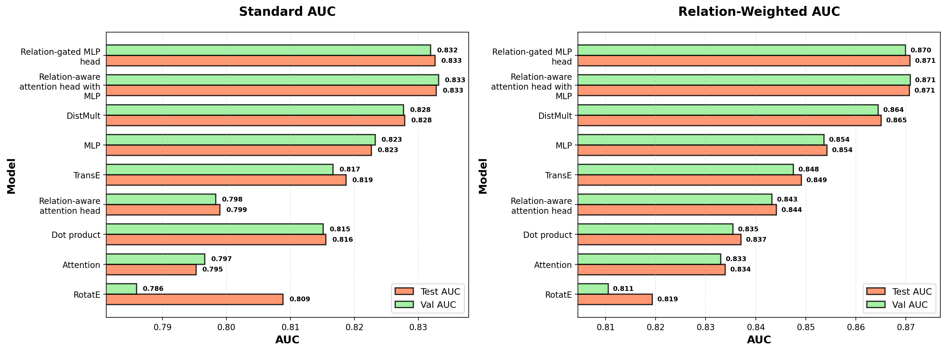
Comparing models with standard and relation-weighted AUC

To evaluate model performance, I use two complementary metrics:

Standard AUC treats all edges equally, measuring how well models discriminate real edges from random negatives across the entire graph.

Relation-weighted AUC accounts for the imbalanced distribution of relation types by:

1. Calculating AUC separately for each relation type (comparing real edges to negative samples of the same relation type)
2. Taking a weighted average of these per-relation AUCs, where weights are proportional to √N (the square root of each relation type’s frequency)

This relation-weighted metric is particularly important given the highly imbalanced distribution of relation types. Some (like “interactor → interactor”) are far more common than others (like “inhibitor → modified”). The √N weighting balances standard AUC (which would weight by N) and equal weighting (which would weight by 1), ensuring rare relation types influence the metric without dominating it. I used relation-weighted AUC for early stopping during training, prioritizing models that perform well across all relation types rather than just the most abundant ones.

# extract and reorder based on test relation-weighted AUC
test_aucs = _extract_metric(run_summaries, "test_relation_weighted_auc")
performance_order = [x for _, x in sorted(zip(test_aucs, run_summaries.keys()))]
performance_ordered_summaries = {k: run_summaries[k] for k in performance_order}
ordered_labels = [
    textwrap.fill(HEAD_DESCRIPTIONS[x]["label"], width=20)  # Adjust width as needed
    for x in performance_order
]

# Create figure with two subplots
fig, (ax1, ax2) = plt.subplots(1, 2, figsize=(16, 6))

# Plot regular AUC on first axis
plot_auc_only(performance_ordered_summaries, ordered_labels, ax=ax1, title="Standard AUC")

# Plot relation-weighted AUC on second axis
plot_auc_only(
    performance_ordered_summaries,
    ordered_labels,
    test_auc_attribute="test_relation_weighted_auc",
    val_auc_attribute="val_relation_weighted_auc",
    title="Relation-Weighted AUC",
    ax=ax2
)

plt.tight_layout()
plt.show()

Performance across relation types

While the relation-weighted AUC provides an overall performance metric, examining AUC for individual relation types reveals how well each model handles specific regulatory mechanisms. Counterintuitively, “interactor → interactor” edges are among the hardest to predict, possibly because the high density of interaction edges creates competing demands on vertex positioning in the embedding space. In contrast, directed regulatory relation types like “stimulator → reactant” and “catalyst → reactant” achieve higher AUCs across most models.

relation_type_aucs = summarize_relation_type_aucs(run_summaries, relation_types)
ordered_experiments = relation_type_aucs.groupby("experiment").sum().sort_values(by="test_auc", ascending=True).index.tolist()
ordered_relation_types = relation_type_aucs.groupby("relation_type").sum().sort_values(by="test_auc", ascending=True).index.tolist()

fig, ax = plot_combined_grouped_barplot(
    relation_type_aucs,
    category_order=ordered_relation_types,
    attribute_order=ordered_experiments,
    value_vars = ["test_auc"],
    figsize = (6, 8)
)
plt.show()

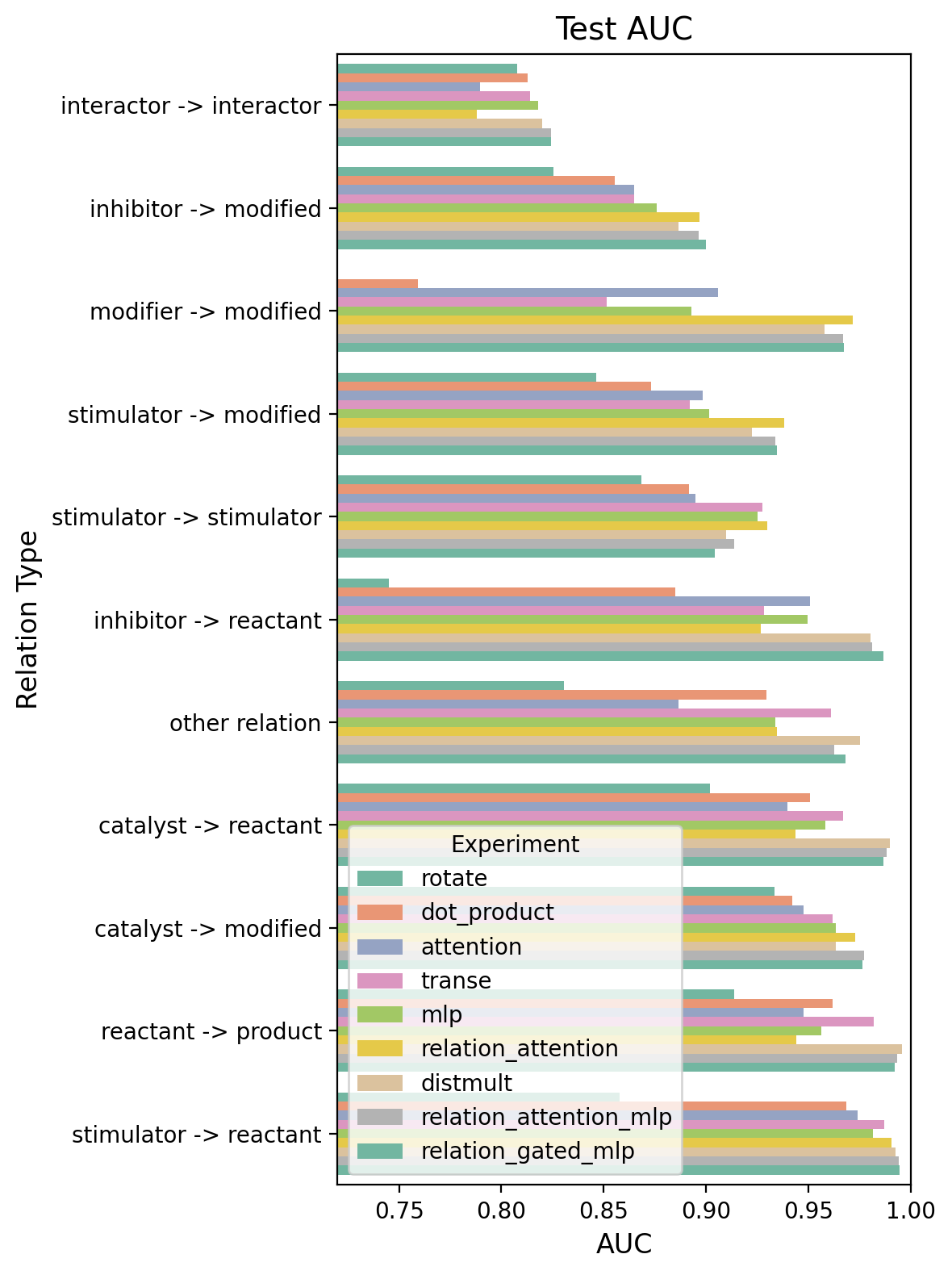
Performance takeaways

Comparing models’ relation-weighted AUC and relation-level AUCs reveals several patterns:

• Expressive relation-aware MLPs achieve top performance. The relation-gated MLP and relation-attention MLP heads achieve nearly equivalent performance (~0.87 relation-weighted AUC), representing the ceiling for this architecture and training regime. Both combine relation-specific modulation with multi-layer MLPs to learn flexible, relation-specific transformations.
• DistMult achieves remarkable parameter efficiency. Despite using only ~1,400 parameters (1/500th of the top MLP heads), DistMult achieves 0.865 relation-weighted AUC, trailing the top models by less than 0.01 AUC points. DistMult learns relation-specific scalar weights for each embedding dimension—the scoring function $\text{score}(h, r, t) = \sum_i h_i \cdot r_i \cdot t_i$ means each relation type re-weights the embedding space to emphasize dimensions where related vertices show correlated (positive weights) or anti-correlated (negative weights) patterns.
• MLPs enable effective vertex attention. Both lightweight attention heads (attention and relation-attention) substantially underperform (0.833-0.844 AUC), barely exceeding dot-product performance. The key architectural difference in top-performing attention-based heads is the MLP that processes concatenated source-target embeddings before attention, creating learned edge feature representations that attention can then modulate. Raw attention over node embeddings alone lacks sufficient expressivity.
• Knowledge graph embedding methods show variable performance. RotatE underperforms relative to even the simple dot-product baseline, likely because treating the 128-dimensional embedding as 64 complex dimensions reduces the vertex representation’s expressivity. TransE performs moderately better but still lags behind custom relation-aware heads. The margin loss used by both methods may be poorly suited for edge prediction—it enforces pairwise rankings between individual positive-negative pairs rather than learning distributional differences between positive and negative edge populations (as BCE loss does). In contrast, DistMult uses BCE loss, and this likely contributes to its strong performance.
• Relation-unaware models show relation-type variation. Even the simple dot-product and MLP heads show varying performance across relation types. This likely reflects competing demands on vertex positioning—vertices involved in many dense interactions (like “interactor → interactor” edges) face more constraints in the embedding space than vertices in sparser relation types. Retraining the dot-product head with relation-weighted BCE (versus standard BCE) substantially shifts the learned embeddings, demonstrating that relation-type frequency affects vertex positioning even when relation type isn’t used as a model input.

Evaluating relation-aware models

To explore whether relation-aware models are making meaningful signed regulatory predictions, I will evaluate them using three analyses:

1. Using interpretable relation-aware knowledge graph embedding heads, I will examine the geometric representation of activation and inhibition in the learned transformations.
2. Exploring top-performing heads, I will examine the strength of regulatory predictions — are scores similar regardless of the putative relation type, or do models confidently predict relation-type-specific interactions?
3. Leveraging PerturbSeq data, I will assess whether models’ top-scoring relation-type predictions (activation vs. inhibition) align with experimentally observed transcriptional responses to genetic perturbations.

What is the geometry of activation and inhibition?

To understand how relation-aware heads encode regulatory semantics, I will examine the learned relation embeddings from three knowledge graph embedding methods: RotatE (rotation angles), TransE (translation vectors), and DistMult (dimensional scaling weights). Each method learns these transformations as model weights, allowing direct inspection of relation types’ geometric encoding.

RotatE_head = models["rotate"].task.head.head
RotatE_phases = RotatE_head.relation_emb.weight.detach().cpu()

TransE_head = models["transe"].task.head.head
TransE_vectors = TransE_head.relation_emb.weight.detach().cpu()

DistMult_head = models["distmult"].task.head.head
DistMult_scalars = DistMult_head.relation_emb.weight.detach().cpu()
DistMult_deviations = DistMult_scalars - 1.0  # Deviation from identity

# Get relation indices
regulatory_relations = {
    "activation": relation_types.index("stimulator -> modified"),
    "inhibition": relation_types.index("inhibitor -> modified"),
    "interaction": relation_types.index("interactor -> interactor"),
}

# Compute relation-type similarity matrices for each method
similarity_matrices = {}
for method_name, embeddings in [
    ("RotatE", RotatE_phases),
    ("TransE", TransE_vectors),
    ("DistMult", DistMult_deviations)
]:
    embeddings_norm = F.normalize(embeddings, p=2, dim=1)
    sim_matrix = embeddings_norm @ embeddings_norm.T
    similarity_matrices[method_name] = sim_matrix

Rather than examining all relation types globally, I will focus on three biologically meaningful questions.

Do stimulators and inhibitors have opposing transformations?

If activation and inhibition are fundamentally opposite processes, their learned embeddings should anti-correlate:

\[r_{\text{stimulator → modified}} \approx -r_{\text{inhibitor → modified}}\]

# Calculate median similarity for context
median_similarities = {}
n_relations = len(relation_types)
mask = np.triu_indices(n_relations, k=1)

for method_name in ["RotatE", "TransE", "DistMult"]:
    sim_flat = similarity_matrices[method_name][mask]
    median_similarities[method_name] = sim_flat.median().item()

stim_vs_inhib = pd.DataFrame({
    "RotatE": [
        similarity_matrices["RotatE"][regulatory_relations["activation"], regulatory_relations["inhibition"]].item(),
        median_similarities["RotatE"]
    ],
    "TransE": [
        similarity_matrices["TransE"][regulatory_relations["activation"], regulatory_relations["inhibition"]].item(),
        median_similarities["TransE"]
    ],
    "DistMult": [
        similarity_matrices["DistMult"][regulatory_relations["activation"], regulatory_relations["inhibition"]].item(),
        median_similarities["DistMult"]
    ]
}, index=["Spearman ρ: activation vs. inhibition", "Spearman ρ: median"])
stim_vs_inhib.index.name = "metric"

pd_utils.format_numeric_columns(stim_vs_inhib, inplace = True)
display_tabulator(
    stim_vs_inhib,
    caption="Reaction-type correlation summaries",
    layout = "fitDataTable",
    include_index=True
)

Reaction-type correlation summaries

Activation and inhibition are not geometric opposites. All three methods show weak or positive correlation rather than the expected anti-correlation. The positive correlations suggest that “being a regulator” is more important than the direction of regulation (activation versus inhibition) in structuring these transformations — both relation types emphasize similar regulatory dimensions rather than encoding opposing effects.

How are undirected relation-types encoded?

Protein-protein interactions are undirected—they exist in the training data as both A → B and B → A edges with the same “interactor → interactor” relation type. One might expect this bidirectional structure to push the relation embedding toward identity (zero rotation, zero translation, unit scaling), which would naturally satisfy:

\[\text{score}(A, r_{\text{interaction}}, B) \approx \text{score}(B, r_{\text{interaction}}, A)\]

To test whether interactor edges learn identity-like transformations, I will extract the learned relation embeddings from each model and compare each relation type’s deviation from identity to the median deviation across all relation types.

interactor_data = {}
for method_name, embeddings in [
    ("RotatE", RotatE_phases),
    ("TransE", TransE_vectors),
    ("DistMult", DistMult_deviations)
]:
    all_magnitudes = embeddings.abs().sum(dim=1)
    median_magnitude = all_magnitudes.median().item()
    interactor_magnitude = all_magnitudes[regulatory_relations["interaction"]].item()
    interactor_data[method_name] = [interactor_magnitude / median_magnitude]

interactor_df = pd.DataFrame(
    interactor_data, 
    index=["interaction transformation norm\n÷\nmedian transformation norm"]
).round(2)
interactor_df.index.name = "metric"

display_tabulator(
    interactor_df,
    caption = "Interaction transformation magnitudes",
    layout = "fitDataTable",
    wrap_columns = {"metric" : "30%"},
    include_index=True
)

Interaction transformation magnitudes

Interactor edges are not near identity. All three methods learn typical or above-median transformations for protein-protein interactions. While this seems to violate the symmetry requirement for undirected edges, the loss functions don’t actually enforce equal scores for A → B and B → A pairs. Instead, they optimize discrimination between real edges and negative samples. For TransE, edges are scored as $\text{score}(h, r, t) = -|h + r - t|$, but the margin-based loss compares these scores to negatives — meaning non-zero transformations can provide discriminative power even without maintaining symmetry.

Do the three methods agree on regulatory semantics?

If all three methods learn similar patterns for how relation types relate to each other, it would suggest they’re converging on shared regulatory semantics.

# Compare similarity matrices pairwise
n_relations = len(relation_types)
mask = np.triu_indices(n_relations, k=1)

agreement_data = {}
for method1, method2 in combinations(similarity_matrices.keys(), 2):
    sim1_flat = similarity_matrices[method1][mask]
    sim2_flat = similarity_matrices[method2][mask]
    rho = compute_spearman_correlation_torch(sim1_flat, sim2_flat, device='cpu')
    agreement_data[f"{method1} vs {method2}"] = [rho]

agreement_df = pd.DataFrame(agreement_data, index=["Spearman ρ"])
agreement_df.index.name = "metric"

pd_utils.format_numeric_columns(agreement_df, inplace = True)
display_tabulator(
    agreement_df,
    caption = "Model-to-model comparison of relation-type correlations",
    layout = "fitDataTable",
    include_index=True
)

Model-to-model comparison of relation-type correlations

The three methods learn different geometric patterns. The weak inter-method correlations show that RotatE, TransE, and DistMult don’t converge on a shared representation of abstract regulatory relationships, instead they learn method-specific solutions to the edge discrimination task.

Geometry summary

The geometric analysis reveals that knowledge graph embedding methods don’t naturally encode biological intuitions about regulatory relationships:

• Activation and inhibition are not geometric opposites, showing weak or positive correlations rather than anti-correlation
• Undirected edges don’t require identity transformations, with interaction edges learning typical or above-median transformation magnitudes despite being bidirectional in the training data
• Methods don’t converge on shared geometric patterns, suggesting they learn different solutions rather than discovering universal principles of abstract biological regulation

The training graph is dense and shaped by experimental ascertainment biases — different relation types are more readily detected for different subsets of vertices. Knowledge graph embedding heads struggle to cleanly separate activators from inhibitors through vertex positioning alone, instead learning transformations that discriminate real edges from negatives without capturing clear regulatory semantics. DistMult’s strong performance despite this limitation is impressive.

Are models predicting relation-specific interactions?

If heads are learning relation-type-specific transformations, edges should score highly for some relation types and poorly for others. If heads rely on vertex embeddings alone, edge scores should remain similar regardless of the assigned relation type.

To evaluate the specificity of relation-type-based scoring, I will score each test set edge under every possible relation type, then calculate the Spearman correlation between relation types’ edge score distributions. High correlations indicate a model assigns similar scores regardless of relation type, while low correlations suggest relation-specific predictions.

if not os.path.exists(CROSS_RELATION_PREDICTION_CACHE):
    cross_relation_prediction_matrices = {"confusion": {}, "correlation": {}}
    for experiment in RELATION_AWARE_FOCUSED_HEADS:
        model = models[experiment]
        cross_relation_prediction_matrices["confusion"][experiment], cross_relation_prediction_matrices["correlation"][experiment] = (
            calculate_relation_type_confusion_and_correlation(model, napistu_data, normalize="true")
        )

    napistu_utils.save_pickle(CROSS_RELATION_PREDICTION_CACHE, cross_relation_prediction_matrices)
else:
    cross_relation_prediction_matrices = napistu_utils.load_pickle(CROSS_RELATION_PREDICTION_CACHE)

fig, axes = plt.subplots(2, 2, figsize=(16, 16))
axes = axes.flatten()

for idx, head in enumerate(RELATION_AWARE_FOCUSED_HEADS):
    correlation_matrix = cross_relation_prediction_matrices["correlation"][head]
    title = textwrap.fill(HEAD_DESCRIPTIONS[head]["label"], width=30)
    plot_heatmap(
        correlation_matrix,
        row_labels=relation_types,
        title=title,
        cmap='magma',
        cbar=False,
        fmt='.2f',
        vmax=1,
        vmin=0,
        cbar_label='Spearman ρ',
        mask_upper_triangle=True,
        square=True,
        cluster='both',
        cluster_method='average',
        cluster_metric='euclidean',
        title_size=22,
        ax=axes[idx],
    )

plt.tight_layout()
plt.show()

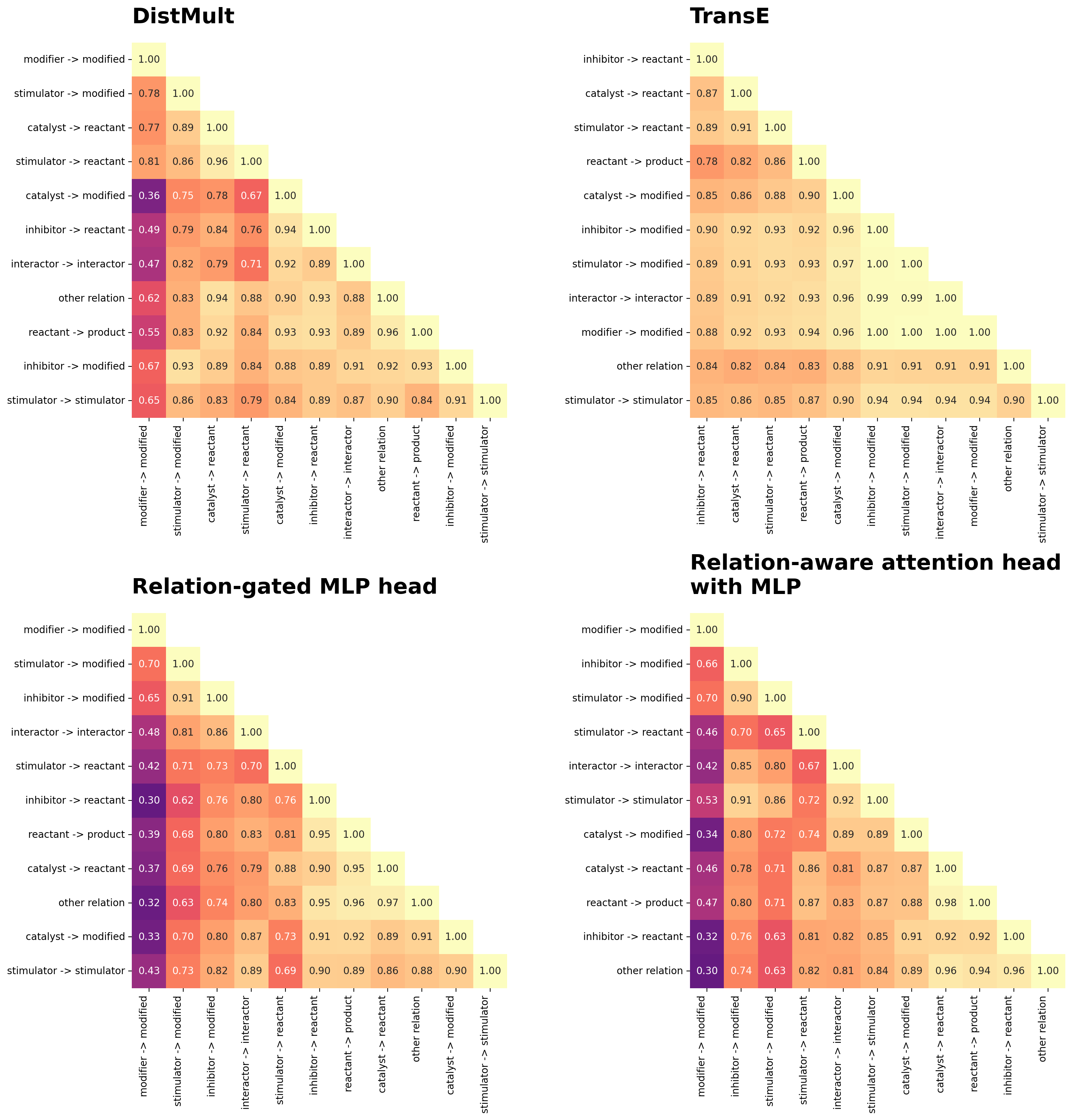
From these cross-relation-type score correlations, several patterns emerge:

• Top-performing models show strong relation-type specificity. DistMult, relation-gated MLP, and relation-attention MLP heads all generate predictions that are highly dependent on relation type, with lower cross-relation correlations indicating distinct scoring patterns for different edge types. This relation-type specificity appears essential for achieving top performance (>0.86 relation-weighted AUC).
• High-performing heads share common structural patterns. The top three model’s relation-type score correlation structures are similar (rho ~= 0.75 DistMult-MLPs, and rho = 0.96 MLP-MLP), suggesting they are learning similar patterns. This is particularly apparent for “modifier → modified” edges, which are distinguished from other relation types. This may reflect a source-specific curation quirk that provides a strong training signal: “modifier → modified” edges arise primarily from a single source (Omnipath) when an interaction is annotated as both activation and inhibition, creating a distinctive pattern that these models learn to recognize.
• TransE shows limited relation-type differentiation. TransE assigns similar scores to edges regardless of relation type, as evidenced by uniformly high cross-relation correlations. This indicates that it relies more heavily on source and target vertex embedding similarity than on the learned relation-specific transformations, potentially incorporating relation-agnostic discriminative signals rather than capturing true regulatory semantics.

Validating signed predictions with PerturbSeq

To evaluate whether relation-aware heads can predict not just interaction existence but regulatory direction (activation vs. inhibition), I need datasets where molecular species are systematically perturbed and their directed impacts on other species are measured. While many such experiments exist, most are either already incorporated into the graph through resources like STRING and IntAct, or haven’t been aggregated at sufficient scale for validation.

PerturbSeq experiments — where genes are perturbed using CRISPR and transcriptome-wide impacts are measured — provide an ideal validation source. Large-scale datasets like Replogle et al. (2022, Cell) perturb many genes, while smaller studies investigate targeted hypotheses (e.g., human mutation knock-ins). However, the original Replogle dataset reports only Anderson-Darling q-values, not signed fold-changes. I therefore turned to Harmonizome, an ongoing effort from the Ma’ayan lab at Mount Sinai to generate and compare diverse gene-centric profiles (Diamant et al., 2025, Nucleic Acids Research). Harmonizome provides signed PerturbSeq fold-changes from both the Replogle datasets and PerturbAtlas in consistent data formats.

To evaluate model predictions against PerturbSeq data, I:

1. Mapped PerturbSeq data to graph vertices. Loaded species identifiers (systematic identifier to molecular species ID mappings) and compartmentalized species ID maps to translate PerturbSeq systematic identifiers into graph vertex IDs.
2. Processed Harmonizome PerturbSeq interactions:
   • Mapped source and target genes to vertex IDs using the adapters from step 1
   • Selected strong perturbations by comparing Harmonizome values to their thresholds
   • Inferred regulatory direction from perturbation type and fold-change direction:
     • Overexpression + upregulation → activation
     • Overexpression + downregulation → inhibition\
     • Knockout/knockdown + upregulation → inhibition (de-repression)
     • Knockout/knockdown + downregulation → activation
     • Other perturbation types (e.g., knock-ins) were excluded
3. Generated relation-type predictions. For each PerturbSeq edge (represented as source-target vertex indices), I scored both activating (“stimulator → modified”) and repressive (“inhibitor → modified”) relation types using each model. I assigned the higher-scoring relation type as the predicted regulatory direction.
4. Compared predictions to PerturbSeq ground truth. I constructed 2×2 contingency tables comparing predicted relation types (activation vs. inhibition) to observed PerturbSeq directions, calculated significance using χ² tests, and quantified the agreement between predicted and observed regulatory directions.

# map relation_types to relation_type indices so we can just score select relation_types
relation_type_indices = {k : i for i, k in enumerate(relation_types)}
focused_relation_type_indices = {k : relation_type_indices[k] for k in PERTURBSEQ_RELATION_TYPES}

# load PerturbSeq results from Harmonizome, map to vertices, and  and filter to strong inhibition and activation
distinct_harmonizome_perturbseq_interactions = (
    load_harmonizome_perturbseq_datasets(LOCAL_HARMONIZOME_DATA_DIR, species_identifiers)
    # rollup to 1 entry per dataset, source, target, and perturbation type
    .pipe(_get_distinct_harmonizome_perturbseq_interactions)
    # filter to only perturbation types where predicted direction is clear (e.g., ignore knock-ins and mutations)
    .query("perturbation_type in @SIGNED_PERTURBATION_TYPES")
    # assign predicted direction (strong inhibition, strong activation)
    .assign(perturbseq_prediction=lambda df: assign_predicted_direction(df))
    .query("perturbseq_prediction in @STRONG_ORDERED_SIGNED_PERTURBSEQ_DIRECTIONS")
)

# pull out all unique from-to species id pairs
distinct_perturbseq_pairs = (
    distinct_harmonizome_perturbseq_interactions[["perturbed_species_id", "target_species_id"]]
    .drop_duplicates()
    .reset_index(drop=True)
)

# Map from species_id to integer_ids and convert to tensor
perturbseq_edgelist_tensor = get_perturbseq_edgelist_tensor(
    distinct_perturbseq_pairs,
    name_to_sid_map
)

# create predictions for the models of interest
predicted_relation_type_vs_perturbseq_truth_predictions = {}
predicted_relation_type_vs_perturbseq_truth_pvalues = {}
for experiment in RELATION_AWARE_FOCUSED_HEADS:
    
    model = models[experiment]

    summaries = compare_relation_type_predictions_to_perturbseq_truth(
        model,
        focused_relation_type_indices,
        perturbseq_edgelist_tensor,
        napistu_data,
        distinct_perturbseq_pairs,
        distinct_harmonizome_perturbseq_interactions,
        STRONG_ORDERED_SIGNED_PERTURBSEQ_DIRECTIONS,
        PERTURBSEQ_RELATION_TYPES,
    )

    predicted_relation_type_vs_perturbseq_truth_predictions[experiment], predicted_relation_type_vs_perturbseq_truth_pvalues[experiment] = summaries

# create the heatmaps

fig, axes = plt.subplots(2, 2, figsize=(10, 10))
axes = axes.flatten()

for idx, head in enumerate(RELATION_AWARE_FOCUSED_HEADS):
    
    dat = predicted_relation_type_vs_perturbseq_truth_predictions[head]
    title = textwrap.fill(HEAD_DESCRIPTIONS[head]["label"], width=25) + "\n" + f"log10p = {predicted_relation_type_vs_perturbseq_truth_pvalues[head].round(2)}"
    row_labels = [textwrap.fill(x, width=20) for x in PERTURBSEQ_RELATION_TYPES]
    col_labels = [textwrap.fill(x, width=10) for x in STRONG_ORDERED_SIGNED_PERTURBSEQ_DIRECTIONS]
    x_label = "PerturbSeq Prediction" if idx >= 2 else None
    y_label = "Top Scoring Relation-Type" if idx % 2 == 0 else None
    
    plot_heatmap(
        dat,
        row_labels=row_labels,
        column_labels=col_labels,
        title=title,
        xlabel=x_label,
        ylabel=y_label,
        cmap='magma',
        fmt='.2f',
        vmin=0.3,
        vmax=0.7,
        cbar_label='Proportion',
        square=True,
        cbar = False,
        title_size=16,
        label_size=16,
        axis_title_size=12,
        annot_size=16,
        ax=axes[idx],
    )

plt.tight_layout()
plt.show()

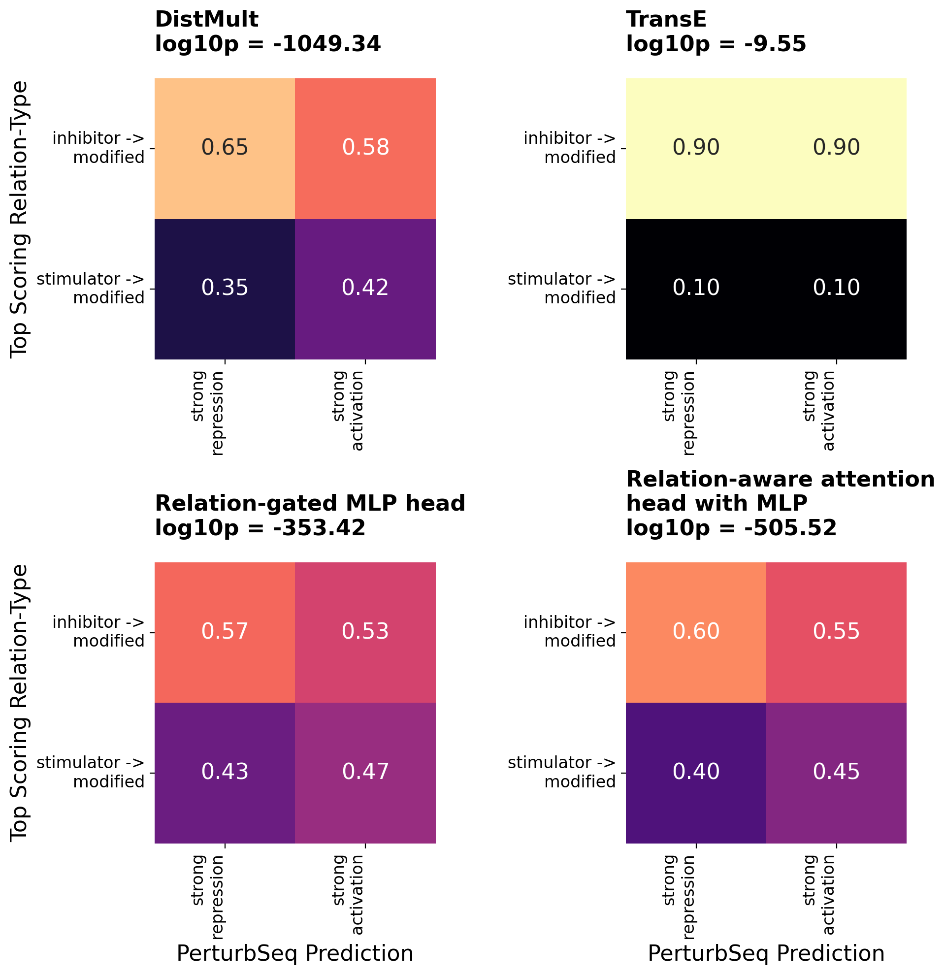
Several patterns emerge from these contingency tables:

• Relation-type scores lack cross-calibration. Average scores can vary substantially between relation types within a model. This is most apparent for TransE, where inhibitory edges score systematically higher than activating edges, resulting in predominantly inhibitory predictions regardless of ground truth. Since the loss function compares real edges to negative samples within the same relation-type stratum, models have no incentive to calibrate scores across relation types.
• TransE predictions are independent of PerturbSeq ground truth. TransE’s top-scoring relation types are only weakly associated with observed regulatory direction (log10p = -2.98). There is actually a slight enrichment in the off-diagonal quadrants (top-right and bottom-left), where predictions disagree with CRISPR results.
• Top-performing relation-aware heads achieve strong agreement with ground truth. All three of the top-performing models (DistMult, the relation-gated MLP and relation-aware attention heads) show striking enrichment along the diagonal (top-left and bottom-right quadrants), indicating correct prediction of regulatory direction. The statistical significance is overwhelming (log10p < -300), with meaningful visual enrichment patterns where predicted activation/inhibition aligns with observed PerturbSeq responses.

The agreement between top-scoring relation types and CRISPR ground truth is particularly impressive given several important caveats:

• Regulatory ground truth is inherently muddy. Harmonizome’s predicted regulatory calls show limited alignment with the Anderson-Darling q-values reported in the original Replogle supplement, highlighting the fundamental difficulty of establishing definitive in vivo regulatory ground truth from experimental data.
• PerturbSeq captures both direct and indirect effects. CRISPRi perturbations measure transcriptome-wide changes that include both immediate regulatory targets and downstream cascade effects. While I’d expect models to predict direct interactions more accurately, the training data itself contains a mixture of direct and indirect interactions, and relation types may provide a means for expressing this distinction.
• Signed regulatory edges are rare in the training data. Activation (“stimulator → modified”) and inhibition (“inhibitor → modified”) edges comprise a small fraction of the graph compared to undirected physical interactions (~3% of edges). The fact that models can accurately distinguish these regulatory directions despite their relative scarcity demonstrates that these concepts are effectively encoded into the vertex and relation-type embeddings.

Published models

All of the data and models used in this analysis are available on Hugging Face.

The best-performing relation-aware models may be of particular interest to others. These are 128-dim GraphConv encoders trained for relation-stratified edge prediction with the following heads:

• DistMult head
• Relation-gated MLP head
• Relation-attention MLP head

Summary

Relation-aware graph neural networks offer a promising path forward for predicting signed regulatory interactions — a major blind spot in current virtual cell modeling efforts. While large-scale single-cell RNA-seq atlases have enabled unprecedented molecular profiling, translating these observations into predictive models of cellular regulation requires distinguishing activation from inhibition, not just identifying that interactions exist.

The results here validate both the expressive, expansive Napistu graphs and the power of mining them with graph neural networks:

• Appropriate architectures matter more than parameter count. Top-performing heads (DistMult, relation-gated MLP, relation-attention MLP) all achieve strong relation-type specificity, but through different mechanisms. DistMult accomplishes this with minimal parameters (~1,400) through dimensional weighting, while MLP-based heads use 60-90K parameters for gating or attention mechanisms. Critically, raw attention heads substantially underperform despite having 20× more parameters than DistMult, demonstrating that architectural choices trump raw model size.
• Learned relation embeddings prioritize discrimination over semantic meaning. Activation and inhibition — biologically opposing processes—produce similar rather than anti-correlated geometric transformations. Undirected edges are not encoded with symmetric transformations that would score A→B and B→A equally. The geometric patterns learned by these methods reflect statistical structure useful for edge discrimination, rather than interpretable regulatory semantics.
• PerturbSeq validation demonstrates biological grounding. Top-performing models show impressive agreement with CRISPR perturbation ground truth, correctly distinguishing activation from inhibition with overwhelming statistical significance (log10p < -300). This validation against orthogonal experimental data confirms the models have learned biologically meaningful representations of regulation.

This work opens several opportunities for refinement. Adapting loss functions to calibrate scores across relation types would enable more interpretable cross-relation comparisons and better support for predicting novel interaction types. Continued architectural innovation in encoder–decoder designs — particularly in how relation information gates or modulates vertex representations — could further improve the semantic encoding of regulatory concepts. These advances would strengthen the foundation for computational models capable of predicting not just molecular associations, but also their functional consequences in cellular systems.