Decoding Virtual Cell Foundation Models II: Cross-Model Attention and Molecular Interactions

The central question motivating this series is whether the attention patterns learned by single-cell foundation models reflect genuine molecular circuits, or whether they are merely recapitulating pairwise co-expression. The distinction matters: co-expression is observational, collapsing direct regulation, shared upstream control, and correlated noise into a single undifferentiated signal. If attention is instead tracking direct regulatory relationships, it becomes causally interpretable, a map of which genes are actually controlling which, grounded in mechanisms that can be perturbed and tested experimentally.

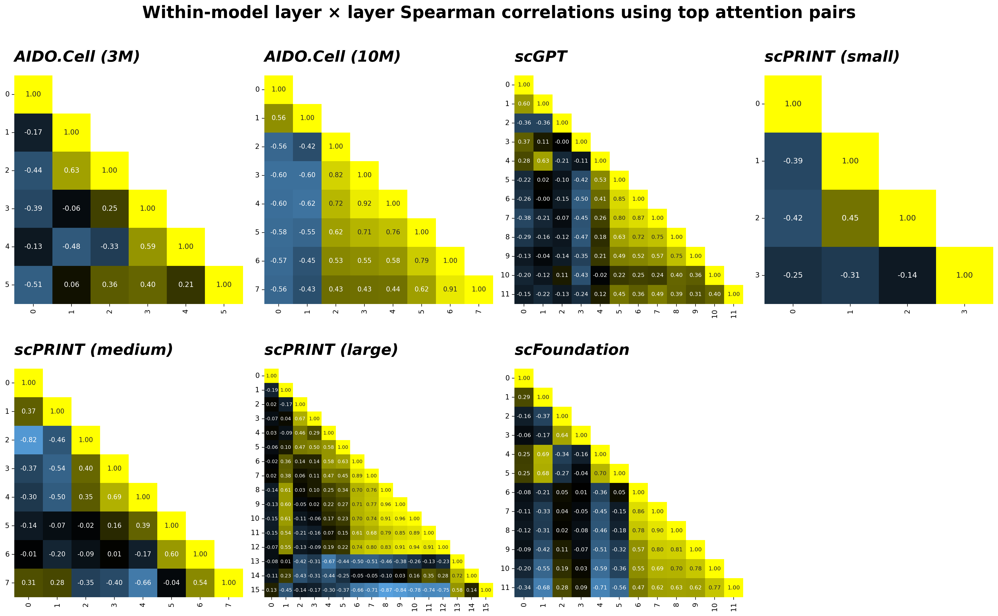
In Part 1, I built a common framework for extracting and comparing attention patterns across four single-cell foundation model families — scGPT, scFoundation, scPRINT, and AIDO.Cell and nearly two orders of magnitude in parameter count. A key finding was that later layers actively suppress the gene-pair structure that early layers establish; early and late attention patterns are often strongly anticorrelated within a model.

Here, I extend the analysis in two directions:

1. Cross-model attention consistency: Do different models converge on the same high-attention gene pairs, even if the overall layer structure differs? I compare the top-K attention pairs across all model × layer combinations to ask whether models converge on a shared set of high-attention pairs despite differences in architecture and training.
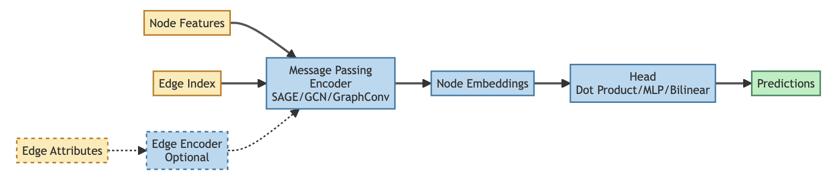
2. Validation against molecular interaction networks: I compare each model’s high-attention pairs to the Napistu Octopus network (50K vertices, 8M edges) and to a GNN trained on self-supervised edge prediction, asking whether attention-highlighted gene pairs are enriched for known regulatory interactions.

Getting started

Reproducing this analysis

This analysis works with the same environment and extracted model summaries (weights, residual streams) from the Part 1 notebook, see the Reproducing this analysis section for details.

To run this notebook:

1. Download the sc_foundation_model_network_interactions.qmd notebook (or copy and paste the relevant code blocks).

2. Configure PROJECT_DIR and other paths in the env_setup code block to point to your local directories.

Configuration and imports

# standard library
import logging
import re
from pathlib import Path
from typing import Dict, List, Optional, Tuple

# 3rd party
import pandas as pd
import numpy as np
import matplotlib.cm as cm
import matplotlib.pyplot as plt
from matplotlib.colors import LinearSegmentedColormap
import seaborn as sns
import torch

# Napistu
from napistu.utils import load_pickle, save_pickle
from napistu.constants import BQB_DEFINING_ATTRS_LOOSE, SBML_DFS
from napistu.network.constants import NAPISTU_GRAPH_EDGES, NAPISTU_GRAPH_VERTICES
from napistu.ontologies.constants import ONTOLOGIES

# Napistu-Torch
from napistu_torch.load.constants import DEFAULT_ARTIFACTS_NAMES
from napistu_torch.evaluation.manager import RemoteEvaluationManager
from napistu_torch.foundation_models.attention_patterns import (
    AttentionPatternsInputs,
    aggregate_embedding_comparisons_over_categories,
    validate_embedding_comparisons_settings,
)
from napistu_torch.foundation_models.foundation_models import (
    FoundationModel,
    FoundationModelStore,
    FoundationModels,
    _get_disk_name,
)
from napistu_torch.foundation_models.constants import (
    COMPARE_EMBEDDINGS_COMPARISONS,
    COMPARE_EMBEDDINGS_SETTINGS,
    FM_EDGELIST,
    FOUNDATION_MODEL_NAMES,
    MODEL_NICE_NAMES,
)
from napistu_torch.napistu_data_store import NapistuDataStore
from napistu_torch.utils.napistu_utils import map_identifiers_to_vertex_names
from napistu_torch.utils.pd_utils import reorder_multindex_by_categorical_and_numeric
from napistu_torch.utils.tensor_utils import compute_cosine_distances_torch
from napistu_torch.visualization.heatmaps import plot_heatmap
from shackett_utils.blog.html_utils import display_tabulator, export_tabulator_payload

logging.basicConfig(level=logging.INFO, format='%(levelname)s:%(name)s:%(message)s')
logger = logging.getLogger(__name__)

# paths
PROJECT_DIR = Path("~/Desktop/DATA/sc_foundation_models").expanduser()
CACHE_DIR = PROJECT_DIR / "cache"
MODEL_OUTPUTS_DIR = PROJECT_DIR / "model_outputs"
STORE_DIR = Path("~/Desktop/EXPERIMENTS/.store").expanduser()

# model inclusion settings
INCLUDE_SCGPT = True
INCLUDE_SCFOUNDATION = False

# analysis settings
CONSENSUS_METHOD = "sum"
BY_ABSOLUTE_VALUE = False
TOP_K = 10000
IGNORE_SELF_ATTENTION = True
OVERWRITE = False
VERBOSE = False
COMPARISON_TYPES = [
    COMPARE_EMBEDDINGS_COMPARISONS.CROSS_MODEL_X_LAYER_TOP_ATTENTIONS,
    COMPARE_EMBEDDINGS_COMPARISONS.CROSS_MODEL_X_LAYER_RANK_AGREEMENT,
]

# general config and constants

IGNORE_CATEGORIES_WITH = ["unknown"]
IGNORED_MODELS = ["AIDOCell_aido_cell_100m"] # not runnable on MPS, just CUDA/flash-attention
HF_GNN_REPOSITORY = "seanhacks/edge_prediction_mlp_256e"
EMBEDDING_DATASET = "efthymiou2025"

MODEL_CATEGORIES = pd.DataFrame([
    {"model type": "scGPT",        "model_category": "scGPT"},
    {"model type": "scPRINT",      "model_category": "scPRINT"},
    {"model type": "scFoundation", "model_category": "GenBioAI"},
    {"model type": "AIDOCell",     "model_category": "GenBioAI"},
])
EXPECTED_NAME_TO_SID_MAP_COLUMNS = {SBML_DFS.S_ID, NAPISTU_GRAPH_VERTICES.NAME}

# blue #1D4A7A, white #F0EDE8, red #C01D2E
bwr = LinearSegmentedColormap.from_list(
    "red_white_blue",
    ["#1D4A7A", "#F0EDE8", "#C01D2E"],  # flip: blue=low, red=high
)

def to_filename(s: str) -> str:
    s = re.sub(r"[^\w\s-]", "", s)
    s = re.sub(r"\s+", "_", s)
    return s.strip("-_")

def get_model_names(
    include_scgpt: bool = True,
    include_scfoundation: bool = True,
    ignored_models: List[str] | None = None,
) -> List[str]:
    ignored = ignored_models or []
    full_names = [
        _get_disk_name(model_name, model_variant)
        for model_name, model_variant in MODEL_NICE_NAMES
        if include_scgpt or model_name != FOUNDATION_MODEL_NAMES.SCGPT
        if include_scfoundation or model_name != FOUNDATION_MODEL_NAMES.SCFOUNDATION
    ]
    if ignored:
        invalid = [name for name in ignored if name not in full_names]
        if invalid:
            logger.warning(f"Ignored models not found in known model names: {invalid}")
        full_names = [name for name in full_names if name not in ignored]
    return full_names

def n_genes_in_dataset_embedding_summary(
    disk_name_or_model: str | FoundationModel,
    model_outputs_dir: Path,
    embedding_dataset: str,
    ignore_categories_with: List[str],
) -> int | str:
    if isinstance(disk_name_or_model, str):
        model = FoundationModel.load(Path(model_outputs_dir) / disk_name_or_model)
        disk_tag = disk_name_or_model
    else:
        model = disk_name_or_model
        disk_tag = model.disk_name

    categories = sorted([
        category
        for category in model.store.list_categories(embedding_dataset)
        if not any(substring in category for substring in ignore_categories_with)
    ])
    if not categories:
        raise ValueError(f"No categories for model {disk_tag!r} in dataset {embedding_dataset!r}")

    counts: List[int] = []
    for category in categories:
        residuals = model.load_category_residuals(embedding_dataset, category)
        counts.append(next(iter(residuals.values())).n_genes)

    uniq = sorted(set(counts))
    if len(uniq) == 1:
        return uniq[0]
    return f"{min(counts)}\u2013{max(counts)}"

def get_model_label_maps(model_metadata_summary: pd.DataFrame) -> Tuple[dict, dict]:
    model_type_map = model_metadata_summary.set_index("model")["model type"].to_dict()
    model_variant_map = model_metadata_summary.set_index("model")["model variant"].to_dict()
    return model_type_map, model_variant_map

OPTIONAL_MODEL_TYPES = (
    FOUNDATION_MODEL_NAMES.SCGPT,
    FOUNDATION_MODEL_NAMES.SCFOUNDATION,
)

def append_missing_optional_model_rows(
    model_metadata_summary: pd.DataFrame,
    optional_model_types: Tuple[str, ...] = OPTIONAL_MODEL_TYPES,
) -> pd.DataFrame:
    if "model type" not in model_metadata_summary.columns:
        return model_metadata_summary

    present_types = set(model_metadata_summary["model type"].astype(str))
    stub_rows = []
    for model_type in optional_model_types:
        if model_type in present_types:
            continue
        label = MODEL_NICE_NAMES.get((model_type, None), model_type)
        row = {column: pd.NA for column in model_metadata_summary.columns}
        row["model"] = label
        row["model type"] = model_type
        stub_rows.append(row)

    if not stub_rows:
        return model_metadata_summary
    return pd.concat([model_metadata_summary, pd.DataFrame(stub_rows)], ignore_index=True)

def mark_optional_model_inclusion(
    model_metadata_summary: pd.DataFrame,
    include_scgpt: bool,
    include_scfoundation: bool,
) -> pd.DataFrame:
    optional_flags = {
        FOUNDATION_MODEL_NAMES.SCGPT: include_scgpt,
        FOUNDATION_MODEL_NAMES.SCFOUNDATION: include_scfoundation,
    }

    def _inclusion_mark(model_type) -> str:
        model_type_str = "" if pd.isna(model_type) else str(model_type).strip()
        if model_type_str in optional_flags:
            return "✅" if optional_flags[model_type_str] else "❌"
        return "✅"

    result = model_metadata_summary.copy()
    result["included"] = result["model type"].apply(_inclusion_mark)
    return result

def get_cache_path(
    dataset: str,
    category: str,
    cache_dir: Path,
    include_scgpt: bool,
    include_scfoundation: bool,
) -> Path:
    scgpt_flag = "with_scgpt" if include_scgpt else "without_scgpt"
    sf_flag = "with_scfoundation" if include_scfoundation else "without_scfoundation"
    return cache_dir / f"cross_model_{dataset}_{to_filename(category)}_{scgpt_flag}_{sf_flag}.pkl"

def summarize_shared_n_genes_over_categories(
    category_summaries: Dict[str, dict],
    include_scfoundation: bool,
) -> int | str:
    counts = [
        summary[COMPARE_EMBEDDINGS_COMPARISONS.SETTINGS][COMPARE_EMBEDDINGS_SETTINGS.N_GENES]
        for summary in category_summaries.values()
    ]
    if not counts:
        raise ValueError("No category summaries to summarize n_genes over")

    lo, hi = min(counts), max(counts)
    if include_scfoundation and lo != hi:
        return f"{lo}\u2013{hi}"
    if len(set(counts)) == 1:
        return counts[0]
    return f"{lo}\u2013{hi}"

def get_all_categories(
    model_outputs_dir: Path,
    embedding_dataset: str,
    ignore_categories_with: List[str],
    include_scgpt: bool,
    include_scfoundation: bool,
    ignored_models: List[str],
) -> List[str]:
    model_names = get_model_names(
        include_scgpt=include_scgpt,
        include_scfoundation=include_scfoundation,
        ignored_models=ignored_models,
    )
    stores = [FoundationModelStore(Path(model_outputs_dir) / name) for name in model_names]
    category_sets = [set(store.list_categories(embedding_dataset)) for store in stores]
    common = category_sets[0].intersection(*category_sets[1:])
    return sorted([
        category
        for category in common
        if not any(substring in category for substring in ignore_categories_with)
    ])

def get_model_comparison_metadata(
    model_outputs_dir: Path,
    embedding_dataset: str,
    ignore_categories_with: List[str],
    include_scgpt: bool = True,
    include_scfoundation: bool = True,
    ignored_models: Optional[List[str]] = None,
) -> dict:
    model_comparison_metadata = dict()

    models = FoundationModels.load_multiple(
        model_outputs_dir,
        get_model_names(
            include_scgpt=include_scgpt,
            include_scfoundation=include_scfoundation,
            ignored_models=ignored_models,
        ),
        verbose=False,
    )
    model_comparison_metadata["model_order"] = models.model_names

    model_metadata_summary = models.get_summary().rename(columns={
        "full_name": "model",
        "model": "model type",
        "variant": "model variant",
        "embed_dim": "# dim",
        "n_layers": "# layers",
        "n_heads": "# heads",
        "parameter_count": "# parameters",
    })

    model_metadata_summary["# genes"] = [
        n_genes_in_dataset_embedding_summary(
            model,
            model_outputs_dir=model_outputs_dir,
            embedding_dataset=embedding_dataset,
            ignore_categories_with=ignore_categories_with,
        )
        for model in models.models
    ]
    model_comparison_metadata["model_metadata_summary"] = model_metadata_summary

    a_category = models.models[0].store.list_categories(embedding_dataset)[0]
    attended_embeddings = AttentionPatternsInputs.from_expression(
        models, embedding_dataset, a_category, verbose=False
    )
    model_comparison_metadata["gene_ids"] = attended_embeddings.common_gene_ids

    return model_comparison_metadata

def get_display_and_active_model_metadata(
    model_outputs_dir: Path,
    embedding_dataset: str,
    ignore_categories_with: List[str],
    include_scgpt: bool,
    include_scfoundation: bool,
    ignored_models: Optional[List[str]] = None,
) -> Tuple[pd.DataFrame, dict]:
    full_metadata = get_model_comparison_metadata(
        model_outputs_dir=model_outputs_dir,
        embedding_dataset=embedding_dataset,
        ignore_categories_with=ignore_categories_with,
        include_scgpt=True,
        include_scfoundation=True,
        ignored_models=ignored_models,
    )
    model_metadata_summary_full = mark_optional_model_inclusion(
        append_missing_optional_model_rows(full_metadata["model_metadata_summary"]),
        include_scgpt=include_scgpt,
        include_scfoundation=include_scfoundation,
    )

    if include_scgpt and include_scfoundation:
        active_metadata = full_metadata
    else:
        active_metadata = get_model_comparison_metadata(
            model_outputs_dir=model_outputs_dir,
            embedding_dataset=embedding_dataset,
            ignore_categories_with=ignore_categories_with,
            include_scgpt=include_scgpt,
            include_scfoundation=include_scfoundation,
            ignored_models=ignored_models,
        )

    return model_metadata_summary_full, active_metadata

def get_model_layer_labels(cross_model_top_attentions: pd.DataFrame) -> pd.DataFrame:
    model_layers_df = cross_model_top_attentions[[FM_EDGELIST.MODEL, FM_EDGELIST.LAYER]].drop_duplicates()
    model_layers_df["label"] = model_layers_df.apply(
        lambda row: f"{row[FM_EDGELIST.MODEL]}-{row[FM_EDGELIST.LAYER]}", axis=1
    )
    return model_layers_df

def summarize_cross_model_attention_coherence(
    model_x_layer_rank_agreement: pd.DataFrame,
    model_sources: pd.DataFrame,
) -> pd.Series:
    return (
        model_x_layer_rank_agreement
        .merge(
            model_sources.rename(columns={"model": "query_model", "model_category": "query_model_category"}),
            on=["query_model"], how="left",
        )
        .merge(
            model_sources.rename(columns={"model": "eval_model", "model_category": "eval_model_category"}),
            on=["eval_model"], how="left",
        )
        .query("query_model_category != eval_model_category")
        .assign(log_quantile=lambda df: -np.log10(df["median_quantile"].clip(upper=0.5) * 2))
        .groupby(["query_model", "query_layer", "category"])["log_quantile"]
        .mean()
        .sort_values(ascending=False)
    )

def add_vertex_names_to_edgelist(
    edgelist: pd.DataFrame,
    gene_to_vertex_map: pd.DataFrame,
) -> pd.DataFrame:
    top_k_with_ids = (
        edgelist
        .merge(
            gene_to_vertex_map
            .rename(columns={ONTOLOGIES.ENSEMBL_GENE: FM_EDGELIST.FROM_GENE, NAPISTU_GRAPH_VERTICES.NAME: "from_vertex"})
            .drop(columns=[SBML_DFS.S_ID]),
            on=FM_EDGELIST.FROM_GENE, how="left",
        )
        .merge(
            gene_to_vertex_map
            .rename(columns={ONTOLOGIES.ENSEMBL_GENE: FM_EDGELIST.TO_GENE, NAPISTU_GRAPH_VERTICES.NAME: "to_vertex"})
            .drop(columns=[SBML_DFS.S_ID]),
            on=FM_EDGELIST.TO_GENE, how="left",
        )
    )
    invalid_edges = top_k_with_ids.isna().any(axis=1)
    if invalid_edges.sum() > 0:
        percent_invalid = (invalid_edges.sum() / len(top_k_with_ids)) * 100
        logger.warning(
            f"Dropping {invalid_edges.sum()} edges ({percent_invalid:.2f}%) which could not be mapped to vertices"
        )
    return top_k_with_ids.loc[~invalid_edges]

def calculate_background_edgelist_metrics(
    napistu_data,
    edge_prediction_task,
    vertex_names: List[str],
) -> Tuple[float, float]:
    gene_vertices = set(napistu_data.get_vertex_indices(vertex_names))
    src = napistu_data.edge_index[0]
    dst = napistu_data.edge_index[1]
    gene_vertices_tensor = torch.tensor(list(gene_vertices), dtype=torch.long)
    src_mask = torch.isin(src, gene_vertices_tensor)
    dst_mask = torch.isin(dst, gene_vertices_tensor)
    num_edges = (src_mask & dst_mask).sum().item()
    background_edge_rate = num_edges / (len(gene_vertices) - 1) ** 2

    all_pairs = pd.MultiIndex.from_product(
        [vertex_names, vertex_names], names=[NAPISTU_GRAPH_EDGES.FROM, NAPISTU_GRAPH_EDGES.TO]
    ).to_frame(index=False)
    all_pairs = all_pairs[all_pairs[NAPISTU_GRAPH_EDGES.FROM] != all_pairs[NAPISTU_GRAPH_EDGES.TO]]
    all_pairs = all_pairs.sample(min(10000, len(all_pairs)))

    background_edge_score = edge_prediction_task.predict_edge_scores(
        napistu_data,
        napistu_data.get_edge_indices(all_pairs, NAPISTU_GRAPH_EDGES.FROM, NAPISTU_GRAPH_EDGES.TO),
    ).mean().numpy()

    return background_edge_rate, background_edge_score

def compare_attention_and_napistu_graphs(
    top_k_attention: pd.DataFrame,
    top_k_attention_edgelist: pd.DataFrame,
    napistu_data,
    edge_prediction_task,
    model_order: List[str],
) -> Tuple[pd.DataFrame, pd.DataFrame]:
    edge_indices = napistu_data.get_edge_indices(top_k_attention_edgelist, "from_vertex", "to_vertex")
    predictions = edge_prediction_task.predict_edge_scores(data=napistu_data, edge_index=edge_indices)

    top_k_attention_edgelist["prediction"] = predictions
    top_k_attention_edgelist["direct_edge_exists"] = napistu_data.has_edges(edge_indices)

    top_k_attention_w_metrics = (
        top_k_attention.reset_index()
        .merge(
            top_k_attention_edgelist[["from_gene", "to_gene", "prediction", "direct_edge_exists"]],
            on=["from_gene", "to_gene"], how="left",
        )
    )

    direct_edge_rate = (
        top_k_attention_w_metrics
        .value_counts(["model", "layer", "category", "direct_edge_exists"])
        .reset_index()
        .pivot(index=["model", "layer", "category"], columns="direct_edge_exists", values="count")
        .fillna(0)
        .assign(true_fraction=lambda df: df[True] / df.sum(axis=1))
        .reset_index()
        .assign(model_name=lambda df: pd.Categorical(df["model"], categories=model_order, ordered=True))
    )

    average_edge_prediction = (
        top_k_attention_w_metrics
        .groupby(["model", "layer", "category"])["prediction"]
        .median()
        .reset_index()
        .assign(model_name=lambda df: pd.Categorical(df["model"], categories=model_order, ordered=True))
    )

    return direct_edge_rate, average_edge_prediction

def plot_metric_by_layer(
    data,
    y_col,
    background_value,
    ylabel,
    model_order,
    model_metadata_summary,
    figsize=(14, 4),
    bar_width=0.6,
    group_gap=2,
):
    model_type_map, model_variant_map = get_model_label_maps(model_metadata_summary)
    fig, ax = plt.subplots(figsize=figsize)

    x_pos_map = {}
    current_x = 0
    model_label_positions = {}

    for model in model_order:
        model_data = data[data["model_name"] == model]
        layers = sorted(model_data["layer"].unique())
        model_start = current_x
        for layer in layers:
            x_pos_map[(model, layer)] = current_x
            current_x += 1
        model_label_positions[model] = (model_start + current_x - 1) / 2
        current_x += group_gap

    for model in model_order:
        model_data = data[data["model_name"] == model]
        for layer, group in model_data.groupby("layer"):
            x = x_pos_map[(model, layer)]
            mean_val = group[y_col].mean()
            min_val = group[y_col].min()
            max_val = group[y_col].max()
            ax.bar(x, mean_val, width=bar_width, color="#aaaaaa", alpha=0.8)
            ax.plot([x, x], [min_val, max_val], color="black", linewidth=1, zorder=5)
            ax.plot([x - 0.15, x + 0.15], [min_val, min_val], color="black", linewidth=1, zorder=5)
            ax.plot([x - 0.15, x + 0.15], [max_val, max_val], color="black", linewidth=1, zorder=5)

    ax.set_xticks([x_pos_map[(model, layer)] for model in model_order
                   for layer in sorted(data[data["model_name"] == model]["layer"].unique())])
    ax.set_xticklabels([str(layer) for model in model_order
                        for layer in sorted(data[data["model_name"] == model]["layer"].unique())],
                       fontsize=7)
    ax.axhline(background_value, color="gray", linestyle=":", linewidth=1.5, zorder=0)
    ax.set_xlabel("Layer")
    ax.set_ylabel(ylabel)
    ax.grid(True, alpha=0.3, axis="y")
    plt.tight_layout()

    y_max = ax.get_ylim()[1]
    y_type = y_max * 1.12
    y_variant = y_max * 1.04
    seen_types = {}

    for model, x_center in model_label_positions.items():
        model_type = model_type_map.get(model, model)
        variant = model_variant_map.get(model)
        if model_type not in seen_types:
            seen_types[model_type] = []
        seen_types[model_type].append(x_center)
        if pd.notna(variant):
            ax.text(x_center, y_variant, variant, ha="center", va="bottom", fontsize=8, color="#555555")

    for model_type, positions in seen_types.items():
        ax.text(np.mean(positions), y_type, model_type, ha="center", va="bottom", fontsize=10, fontweight="bold")

    return fig, ax

def plot_stacked_histogram(ax, df, score_col, x_min, x_max, n_bins=40):
    bin_edges = np.linspace(x_min, x_max, n_bins + 1)
    bin_centers = (bin_edges[:-1] + bin_edges[1:]) / 2
    width = bin_edges[1] - bin_edges[0]

    no_edge = df[~df["direct_edge_exists"]][score_col]
    has_edge = df[df["direct_edge_exists"]][score_col]
    no_edge_counts, _ = np.histogram(no_edge, bins=bin_edges)
    has_edge_counts, _ = np.histogram(has_edge, bins=bin_edges)

    ax.bar(bin_centers, has_edge_counts, width=width, label="Direct edge", alpha=0.8, color="#444444")
    ax.bar(bin_centers, no_edge_counts, width=width, bottom=has_edge_counts, label="No direct edge", alpha=0.8, color="#cccccc")

    medians = [(False, "No edge median", "--"), (True, "Direct edge median", "-.")]
    meds = [(df[df["direct_edge_exists"] == exists][score_col].median(), label, linestyle)
            for exists, label, linestyle in medians]
    meds_sorted = sorted(meds, key=lambda item: item[0])
    y_positions = [0.97, 0.83] if len(meds_sorted) == 2 else [0.97]

    for (med, label, linestyle), y_pos in zip(meds_sorted, y_positions):
        ax.axvline(med, linestyle=linestyle, linewidth=1.5, color="gray")
        ax.text(med + 0.01, y_pos, f"{label}: {med:.2f}",
                transform=ax.get_xaxis_transform(), fontsize=8, va="top")

    ax.set_xlabel(score_col.capitalize())
    ax.set_ylabel("Count")
    ax.legend(fontsize=8)
    sns.despine(ax=ax)

def summarize_edgelist_cosine_similarity(
    top_k_attention: pd.DataFrame,
    top_k_attention_edgelist: pd.DataFrame,
    napistu_data,
    napistu_gnn,
    model_order: List[str],
) -> Tuple[pd.DataFrame, float]:
    vertex_names = pd.concat([
        top_k_attention_edgelist["from_vertex"],
        top_k_attention_edgelist["to_vertex"],
    ]).unique().tolist()
    vertex_indices = napistu_data.get_vertex_indices(vertex_names)
    cosine_sim = 1 - compute_cosine_distances_torch(napistu_gnn.get_embeddings(napistu_data)[vertex_indices])
    vertex_to_idx = {name: i for i, name in enumerate(napistu_data.get_vertex_names()[vertex_indices])}

    from_idx = top_k_attention_edgelist["from_vertex"].map(vertex_to_idx)
    to_idx = top_k_attention_edgelist["to_vertex"].map(vertex_to_idx)

    working = top_k_attention_edgelist.copy()
    working["cosine_sim"] = cosine_sim[from_idx.values, to_idx.values]

    average_cosine_sim = (
        top_k_attention.reset_index()
        .merge(working, on=["from_gene", "to_gene"], how="inner")
        .groupby(["model", "layer", "category"])["cosine_sim"]
        .median()
        .reset_index()
        .assign(model_name=lambda df: pd.Categorical(df["model"], categories=model_order, ordered=True))
    )

    return average_cosine_sim, cosine_sim.mean()

def top_attention_to_napistu_edgelist(
    cross_model_top_attentions: pd.DataFrame,
    gene_to_vertex_map: pd.DataFrame,
    top_k: int,
) -> Tuple[pd.DataFrame, pd.DataFrame]:
    top_k_attention = (
        cross_model_top_attentions
        .query("attention_rank <= @top_k")
        .set_index(["model", "layer"])
        .sort_values("attention_rank")
        .sort_index()
    )
    top_k_attention_distinct_edges = top_k_attention[["from_gene", "to_gene"]].drop_duplicates()
    top_k_attention_edgelist = add_vertex_names_to_edgelist(top_k_attention_distinct_edges, gene_to_vertex_map)
    return top_k_attention, top_k_attention_edgelist

Building the cache

For each cell-type cluster and model, I identified the top-10,000 attention pairs at each layer and evaluated how those pairs rank in every other model’s attention distribution at every other layer. Results were cached to disk and aggregated across cell-type clusters.

all_categories = get_all_categories(
    model_outputs_dir=MODEL_OUTPUTS_DIR,
    embedding_dataset=EMBEDDING_DATASET,
    ignore_categories_with=IGNORE_CATEGORIES_WITH,
    include_scgpt=INCLUDE_SCGPT,
    include_scfoundation=INCLUDE_SCFOUNDATION,
    ignored_models=IGNORED_MODELS,
)

scgpt_and_scfoundation_runs = [(True, False), (False, True), (False, False), (True, True)] # populate data for all notebook variants

for include_scgpt, include_scfoundation in scgpt_and_scfoundation_runs:
    for category in all_categories:
        cache_path = get_cache_path(
            EMBEDDING_DATASET,
            category,
            cache_dir=CACHE_DIR,
            include_scgpt=include_scgpt,
            include_scfoundation=include_scfoundation,
        )

        if cache_path.is_file() and not OVERWRITE:
            if VERBOSE:
                logger.info(f"Skipping {category}, cache exists at {cache_path}")
            continue

        logger.info(f"Running {category} with scGPT={include_scgpt} and scFoundation={include_scfoundation}")
        
        model_prefixes = get_model_names(
            include_scgpt,
            include_scfoundation=include_scfoundation,
            ignored_models=IGNORED_MODELS,
        )
        models_subset = FoundationModels.load_multiple(MODEL_OUTPUTS_DIR, model_prefixes, verbose=False)

        attention_patterns_inputs = AttentionPatternsInputs.from_expression(
            models_subset, EMBEDDING_DATASET, category
        )
        comparisons = attention_patterns_inputs.compare(
            top_k=TOP_K,
            comparison_types=COMPARISON_TYPES,
            consensus_method=CONSENSUS_METHOD,
            by_absolute_value=BY_ABSOLUTE_VALUE,
            ignore_self_attention=IGNORE_SELF_ATTENTION,
            verbose=VERBOSE,
        )
        save_pickle(cache_path, comparisons)

        del attention_patterns_inputs, comparisons, models_subset

Loading and aggregating

Cached results are loaded and summarized across cell-type clusters, producing layer-indexed cross-model rank agreement scores used in the analyses below.

# summaries of models under consideration
model_metadata_summary_full, model_comparison_metadata = get_display_and_active_model_metadata(
    model_outputs_dir=MODEL_OUTPUTS_DIR,
    embedding_dataset=EMBEDDING_DATASET,
    ignore_categories_with=IGNORE_CATEGORIES_WITH,
    include_scgpt=INCLUDE_SCGPT,
    include_scfoundation=INCLUDE_SCFOUNDATION,
    ignored_models=IGNORED_MODELS,
)
model_order = model_comparison_metadata["model_order"]

# load and aggregate comparisons
category_summaries = dict()
for category in all_categories:
    cache_path = get_cache_path(
        EMBEDDING_DATASET,
        category,
        cache_dir=CACHE_DIR,
        include_scgpt=INCLUDE_SCGPT,
        include_scfoundation=INCLUDE_SCFOUNDATION,
    )
    category_comparisons = load_pickle(cache_path)
    validate_embedding_comparisons_settings(
        category_comparisons, TOP_K, CONSENSUS_METHOD, BY_ABSOLUTE_VALUE, IGNORE_SELF_ATTENTION, model_order
    )
    category_summaries[category] = category_comparisons

comparisons = aggregate_embedding_comparisons_over_categories(category_summaries)

Foundation models converge on a shared set of high-attention gene pairs

If the attention patterns learned by these models reflect genuine regulatory biology rather than architecture-specific artifacts, independently trained models should converge on similar high-attention gene pairs. Testing this requires a shared vocabulary: scGPT uses gene symbols while the remaining models use Ensembl IDs, and each model covers a different subset of the transcriptome. AttentionPatternsInputs.from_expression() handles the alignment by finding the gene intersection across all models and reordering each model’s embeddings to a common index before computing any cross-model statistics.

display_tabulator(
    model_metadata_summary_full,
    layout="fitDataTable",
    include_index=False,
)

Cross-model comparison requires a common gene vocabulary, which introduces a meaningful tradeoff. A model with a smaller vocabulary may appear to perform better simply because it is already focused on genes central to core biological processes - a form of implicit HVG selection. To avoid this bias, all models are compared over their shared gene intersection, which means genome-scale models like scPRINT and AIDO.Cell have their attention patterns pared down to the common vocabulary.

The models differ substantially in vocabulary size: scGPT operates on the top 1,200 highly variable genes, scFoundation restricts its vocabulary to genes expressed in each cell type (typically 5,000-10,000), and scPRINT and AIDO.Cell embed 18,000-19,000 genes. Including scGPT or scFoundation therefore dramatically reduces the shared vocabulary. To keep comparisons robust, I ran several versions of this notebook that differ only in which models were included; scPRINT and AIDO.Cell are always present, while scGPT and scFoundation are optional. Results are consistent across versions.

This version includes scGPT but excludes scFoundation, comparing models over a shared vocabulary of 744 genes constrained by scGPT’s HVG selection.

Comparing attention patterns across models

In Part 1, I explored how attention patterns evolve across layers within each model, finding that later layers often actively suppress early attention patterns and that cross-layer consistency varies substantially by architecture and model size. These are properties of the models themselves, revealing more about how each architecture processes information than about the biology being captured. The natural next question is whether any of this internal structure reflects something shared: do different architectures converge on the same high-attention gene pairs, even when their architecture, training data, vocabulary, and scale differ?

To test this, I applied the same rank-agreement metric used for within-model comparisons, now across model-layer pairs. For each model and layer, the top-K attention pairs were selected and their median quantile was evaluated against every other model’s layers. High quantile scores indicate that a pair ranked highly in one model also ranks highly in another. Where this coherence is strong, the underlying gene-gene relationship is robustly learned regardless of architecture; where it is weak, it may reflect architecture-specific routing, noise, or simply that the models are capturing different aspects of a complex regulatory landscape.

cross_model_top_attentions = comparisons["cross_model_x_layer_top_attentions"]
model_x_layer_rank_agreement = comparisons["cross_model_x_layer_rank_agreement"]

model_layers_df = get_model_layer_labels(cross_model_top_attentions)
model_layer_labels = model_layers_df["label"].tolist()

conditional_quantiles = (
    model_x_layer_rank_agreement
    # convert from rank quantiles (0 is strongest agreement) to ordinary quantiles (1 indicates the strongest agreement)
    .assign(median_quantile=lambda x: 1 - x["median_quantile"])
    .pivot_table(
        index=["query_model", "query_layer"],
        columns=["eval_model", "eval_layer"],
        values="median_quantile",
        aggfunc="median",
    )
)

reordered_index = reorder_multindex_by_categorical_and_numeric(
    conditional_quantiles.index,
    categorical_order=model_order,
    categorical_level=0,
    numeric_level=1,
)

conditional_quantiles = conditional_quantiles.reindex(
    index=reordered_index,
    columns=reordered_index,
)

model_col_values = conditional_quantiles.columns.get_level_values(0)
mask = model_col_values.to_numpy()[:, None] == model_col_values.to_numpy()[None, :]

plot_heatmap(
    conditional_quantiles,
    row_labels=model_layer_labels,
    suptitle="Cross-model x layer attention consistency",
    title="Median quantiles of top attention pairs from another\nmodel x layer. Within-model attention is masked.",
    xlabel="Evaluated model & layer",
    ylabel="TopK model & layer",
    cmap=bwr,
    cbar=True,
    fmt='.2f',
    vmax=1,
    vmin=0,
    cbar_label='Median rank',
    mask=mask,
    mask_upper_triangle=False,
    mask_color='lightgray',
    annot=False,
    square=True,
    suptitle_size=18,
    title_size=16,
    axis_title_size=16,
    tick_label_size=5,
    title_fontstyle="italic",
    title_fontweight="normal",
    figsize=(9, 9),
)

plt.show()

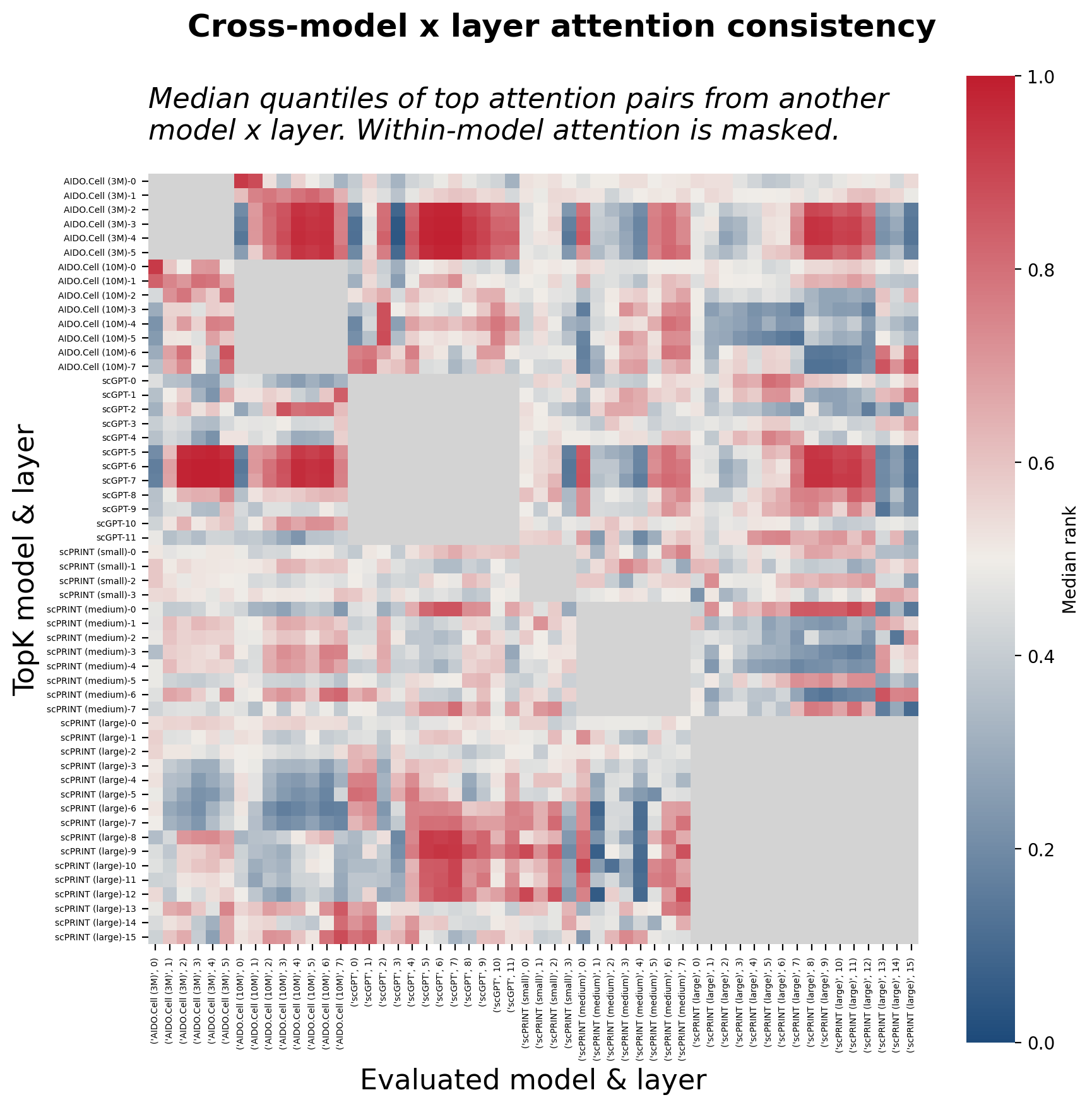
The cross-model consistency matrix reveals that agreement is neither uniform nor random. The strongest cross-model coherence emerges between intermediate layers of scGPT, AIDO.Cell (3M), and scPRINT (large), with their top attention pairs ranking consistently highly in each other’s distributions and forming visible hotspots in the off-diagonal blocks. The other scPRINT variants and AIDO.Cell (10M) show weaker cross-model signals. That three architectures, trained on different objectives, spanning nearly two orders of magnitude in parameter count, converge on overlapping sets of high-attention gene pairs in specific layers is an encouraging signal; it suggests that these pairs reflect structure in the expression data that multiple models independently find useful, rather than artifacts of any particular training run.

Grounding attention patterns in molecular interaction networks

To evaluate whether high-attention gene pairs overlap with known molecular interactions, I mapped each pair against the 8-source Octopus network (~4M reported interactions across 50K proteins, metabolites, and complexes) to compute a reported edge rate, and scored each pair using a GNN trained on self-supervised edge prediction over the same network to obtain a continuous interaction plausibility score. Both measures are reported relative to a vocabulary-matched null (the expected values computed over all gene pairs within the observed vocabulary) since hub genes with high local edge density would inflate raw rates regardless of whether attention is specifically tracking interactions.

napistu_data_store = NapistuDataStore(STORE_DIR)
species_identifiers = (
    napistu_data_store.load_pandas_df(DEFAULT_ARTIFACTS_NAMES.SPECIES_IDENTIFIERS)
    .query("bqb in @BQB_DEFINING_ATTRS_LOOSE")
)
name_to_sid_map = napistu_data_store.load_pandas_df(DEFAULT_ARTIFACTS_NAMES.NAME_TO_SID_MAP).reset_index()

# load the Napistu Edge Prediction MLP
evaluation_manager = RemoteEvaluationManager.from_huggingface(
    HF_GNN_REPOSITORY,
    data_store_dir=STORE_DIR,
)
napistu_gnn = evaluation_manager.load_model_from_checkpoint()
napistu_data = evaluation_manager.load_napistu_data()

# reload cross-model attention data and align gene IDs to Napistu vertices
model_x_layer_rank_agreement = comparisons["cross_model_x_layer_rank_agreement"]
cross_model_top_attentions = comparisons["cross_model_x_layer_top_attentions"]
model_metadata_summary = model_comparison_metadata["model_metadata_summary"]
gene_ids = model_comparison_metadata["gene_ids"]
model_order = model_comparison_metadata["model_order"]

gene_to_vertex_map = map_identifiers_to_vertex_names(gene_ids, species_identifiers, name_to_sid_map)

model_sources = MODEL_CATEGORIES.merge(model_metadata_summary, on=["model type"], how="inner")[["model", "model_category"]]
cross_model_attention_coherence = summarize_cross_model_attention_coherence(model_x_layer_rank_agreement, model_sources)

top_k_attention, top_k_attention_edgelist = top_attention_to_napistu_edgelist(
    cross_model_top_attentions, gene_to_vertex_map, top_k=TOP_K
)

direct_edge_rate, average_edge_prediction = compare_attention_and_napistu_graphs(
    top_k_attention, top_k_attention_edgelist, napistu_data, napistu_gnn.task, model_order
)

background_edge_rate, background_edge_score = calculate_background_edgelist_metrics(
    napistu_data, napistu_gnn.task, gene_to_vertex_map["name"]
)

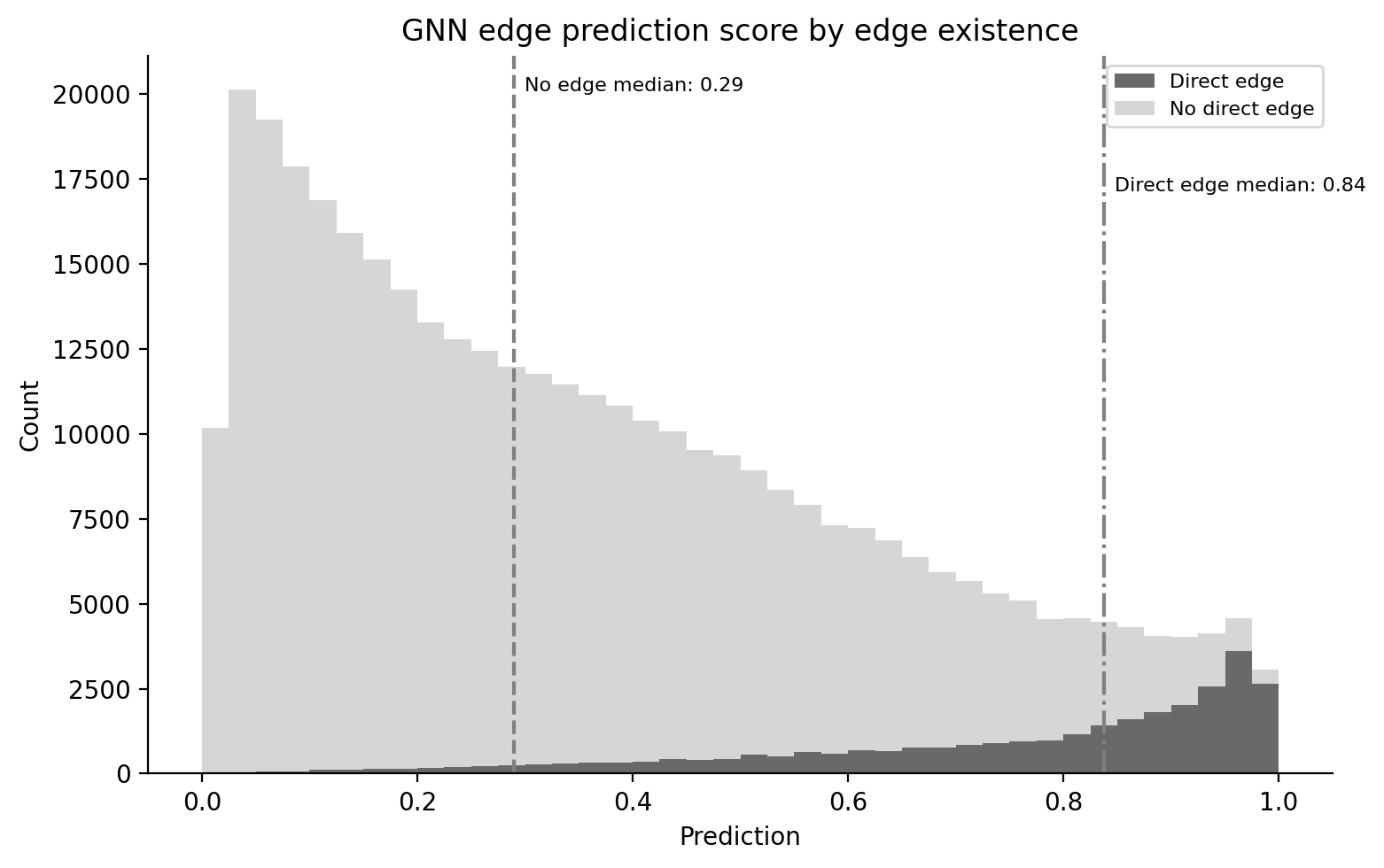
The GNN was trained to predict edge existence in the Octopus network, so its scores are naturally calibrated to that task. The figure below confirms the expected separation: gene pairs with a direct reported interaction score with a median of 0.84, while pairs without one score 0.29. With ~4M edges among ~20K genes, the Octopus network is dense by regulatory network standards but still covers only a small fraction of possible pairs. The GNN score provides a useful continuous signal for the remaining pairs, interpolating interaction plausibility beyond what binary edge existence alone can capture.

fig, ax = plt.subplots(figsize=(8, 5))
plot_stacked_histogram(ax, top_k_attention_edgelist, "prediction", x_min=0, x_max=1)
ax.set_title("GNN edge prediction score by edge existence")
plt.tight_layout()
plt.show()

Interaction enrichment is strong but highly layer-dependent

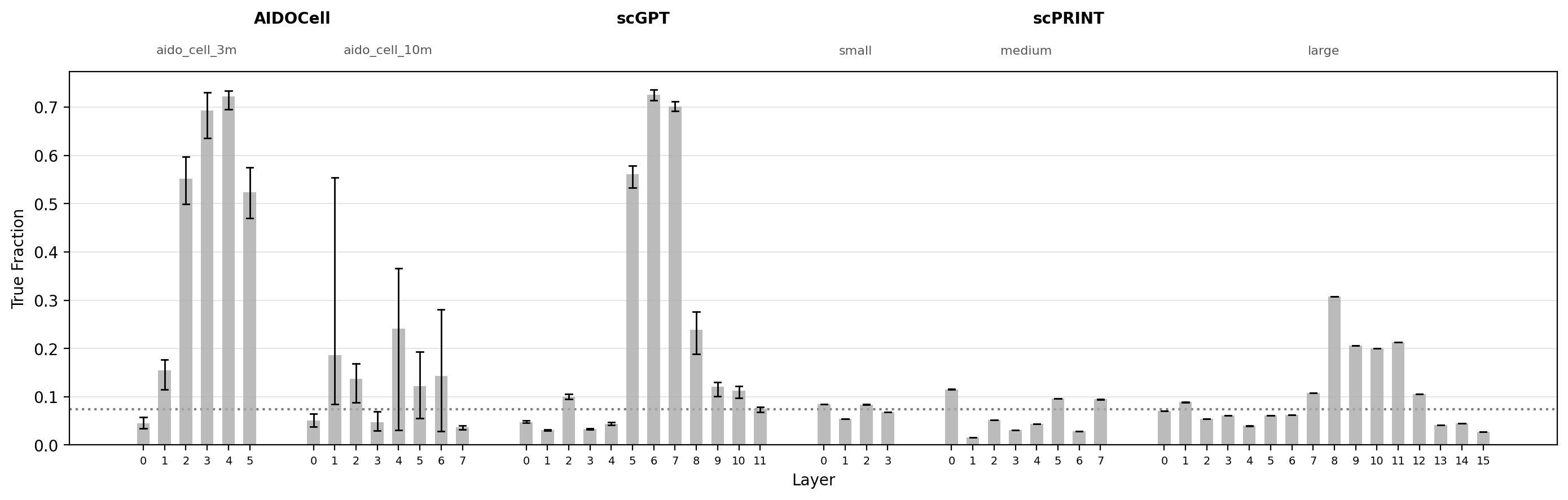
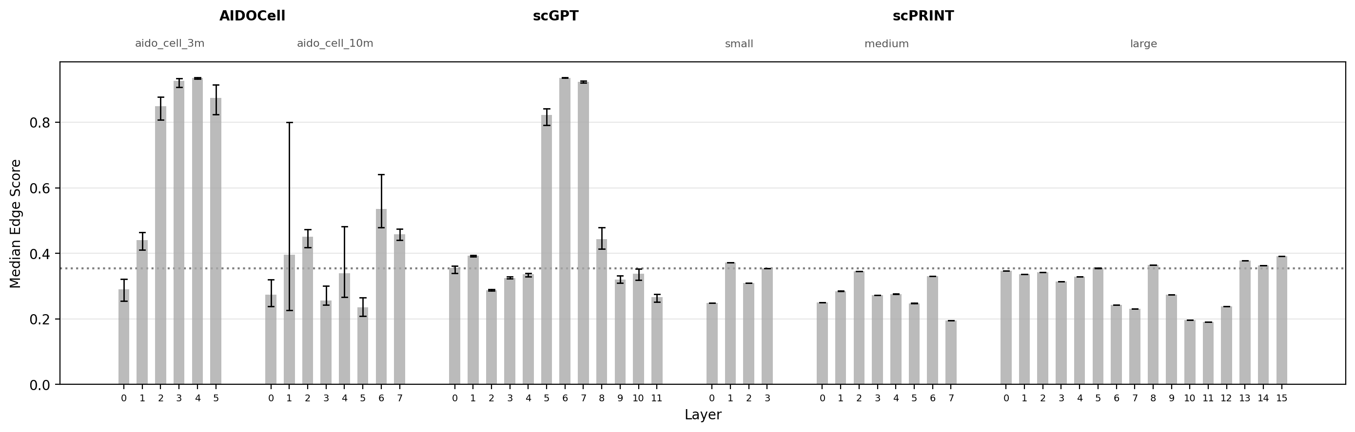
To assess whether attention patterns are enriched for reported and high-scoring interactions, I computed the edge rate and median GNN score for the top-K attention pairs at each model and layer. Since both measures were calculated separately for each cell-type cluster, the range across clusters is shown as a line range.

fig, ax = plot_metric_by_layer(
    data=direct_edge_rate,
    y_col='true_fraction',
    background_value=background_edge_rate,
    ylabel='True Fraction',
    model_order=model_order,
    model_metadata_summary=model_metadata_summary,
)

fig, ax = plot_metric_by_layer(
    data=average_edge_prediction,
    y_col='prediction',
    background_value=background_edge_score,
    ylabel='Median Edge Score',
    model_order=model_order,
    model_metadata_summary=model_metadata_summary,
)

Three patterns stand out:

• Striking enrichment in intermediate layers of scGPT and AIDO.Cell (3M): more than 50% of top-10,000 attention pairs correspond to reported molecular interactions at peak layers, substantially above the vocabulary-matched null.
• Enrichment peaks at intermediate layers across most models: consistent with the conventional interpretation that early layers adapt raw expression to a useful embedding, intermediate layers capture general regulatory structure, and late layers specialize toward cell-type-specific states.

• scPRINT (large) shows a dissociation between edge rate and GNN score: edge rates are above null at several layers, suggesting genuine recovery of reported interactions, but GNN scores remain consistently below the null. Understanding why requires looking more closely at the structure of the attention pairs themselves.

  scFoundation's near-null interaction recovery (as seen in the companion notebook with scFoundation included) likely reflects a fundamental architectural constraint rather than a failure of the model itself. Its asymmetric encoder-decoder design processes only expressed genes through the encoder, recombining those representations with zero-expressed gene embeddings only at the decoder stage to produce final gene-level representations. The residual streams extracted here come from the encoder alone, which has never attended over the full transcriptome. The regulatory signal in scFoundation is probably concentrated in the decoder outputs, but the decoder is closed source, making this analysis of the encoder the limit of what is publicly accessible. This is worth keeping in mind when comparing scFoundation to the other models here, all of which expose their full forward pass.

scPRINT attention preferentially connects mechanistically distant genes

High-attention gene pairs in the largest scPRINT model tend to have low GNN scores despite being enriched for reported interactions. The GNN scores edges using a standard edge prediction MLP applied to source and target vertex embeddings, so low scores could reflect two distinct sources: the MLP penalizing certain interaction types, or the attended pairs being dissimilar in the underlying vertex embedding space. These are meaningfully different — the first implicates the scoring function, the second implicates the structure of the pairs themselves. Vertex embeddings in the Napistu GNN are learned from network topology, so genes with similar local interaction neighborhoods end up close in embedding space; dissimilar embeddings imply genes from different parts of the interaction network, with few shared neighbors. To distinguish between the two explanations, I compared the cosine similarity between source and target vertex embeddings for high-attention pairs across all models against the background distribution of vocabulary-matched pairs.

average_embedding_cosine_similarity, background_embedding_cosine_similarity = summarize_edgelist_cosine_similarity(
    top_k_attention, top_k_attention_edgelist, napistu_data, napistu_gnn, model_order
)

fig, ax = plot_metric_by_layer(
    data=average_embedding_cosine_similarity,
    y_col='cosine_sim',
    background_value=background_embedding_cosine_similarity,
    ylabel='Average vertex embedding cosine similarity\nbetween from-to high-attention pairs',
    model_order=model_order,
    model_metadata_summary=model_metadata_summary,
)

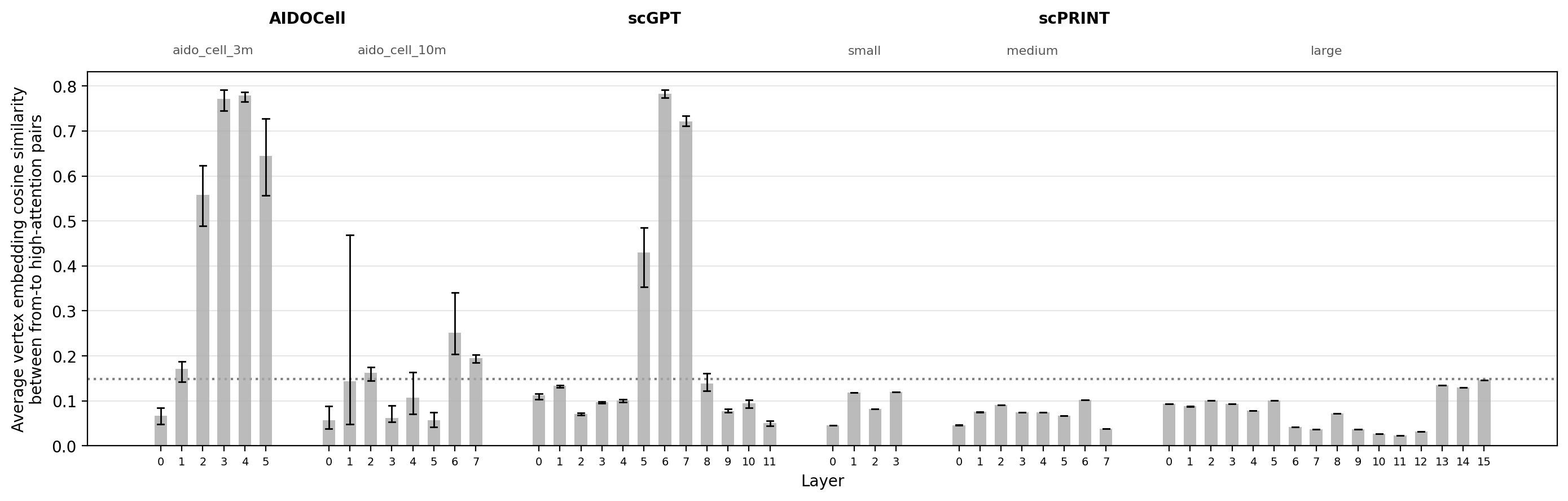
The cosine similarity results reveal a clear split across models. AIDO.Cell (3M) and scGPT intermediate layers attend preferentially to genes that are similar in the GNN embedding space, well above the vocabulary-matched null, consistent with their high edge rates and GNN scores. The largest scPRINT model is the mirror image: high-attention pairs are consistently below the null in cosine similarity throughout all layers, confirming that the low GNN scores reflect genuine dissimilarity in vertex embedding space rather than a scoring artifact from the MLP head.

Taken together, the largest scPRINT model is capturing mechanistically meaningful attention patterns, but biased toward cross-pathway interactions between genes with dissimilar local network neighborhoods. Two factors may contribute:

• Cross-pathway crosstalk provides a stronger learning signal: genes from different pathways interact rarely and specifically, making those pairs more distinctive and easier for the model to learn than the dense, redundant co-expression structure within pathways.
• Within-pathway attention is diluted across many pairs: because co-regulated genes form tight clusters, many pairs are roughly equally plausible candidates for attention, spreading weight across a large number of edges rather than concentrating it on a few, pushing any individual within-pathway pair below the top-K threshold.

The cross-pathway attention bias in scPRINT may be directly attributable to its training objective. Unlike scGPT and AIDO.Cell, which are trained purely on self-supervised expression denoising, scPRINT optimizes a joint loss that includes hierarchical label prediction, classifying cell type, tissue, disease, and other metadata from disentangled cell embeddings. Cell identity is inherently a cross-pathway phenomenon: the features that distinguish cell types span metabolic, cytoskeletal, signaling, and transcriptional programs simultaneously. Attention patterns bridging pathway boundaries are directly rewarded by this classification signal, whereas scGPT and AIDO.Cell are steered toward the block-diagonal co-expression structure that is the optimal strategy for local gene imputation.

It is worth noting that this analysis aggregates attention across all heads equally, whereas scPRINT’s published gene network extraction performs post-hoc head selection based on recovery of known interactions from OmniPath before aggregating. This is an inference-time decision layered on top of the trained model rather than part of the training objective itself, but it would specifically enrich for heads capturing dense within-pathway interactions, potentially reversing the cross-pathway bias observed here. The head-agnostic view taken in this analysis and the head-selected view in the original scPRINT paper may therefore be capturing complementary aspects of what the model has learned.

Layers with strong cross-model coherence are enriched for known and GNN-supported interactions

The preceding analyses established two layer-dependent properties: cross-model attention coherence, where intermediate layers of certain models converge on shared gene pairs, and interaction enrichment, where those same layers show the highest edge rates and GNN scores. Comparing these directly asks whether cross-model coherence is a useful proxy for mechanistic signal, specifically whether the layers where models agree are also those most enriched for known regulatory interactions. Each point represents a single model, layer, and cell-type cluster combination, giving a fine-grained view of how coherence and enrichment co-vary across the full range of model depth and cellular context.

df1 = average_edge_prediction.merge(
    cross_model_attention_coherence,
    left_on=["model", "layer", "category"],
    right_index=True,
)

df2 = direct_edge_rate.merge(
    cross_model_attention_coherence,
    left_on=["model", "layer", "category"],
    right_index=True,
)

models = pd.concat([df1["model"], df2["model"]]).unique()
colors = cm.tab10(np.linspace(0, 1, len(models)))
color_map = dict(zip(models, colors))

fig, axes = plt.subplots(1, 2, figsize=(16, 6))

for ax, df, ylabel in zip(axes, [df1, df2], ["prediction", "true_fraction"]):
    for model, group in df.groupby("model"):
        ax.scatter(
            group["log_quantile"], group[ylabel],
            color=color_map[model], label=model, alpha=0.6, s=20,
        )
    ax.set_xlabel("log_quantile")
    ax.set_ylabel(ylabel)

handles, labels = axes[0].get_legend_handles_labels()
fig.legend(handles, labels, bbox_to_anchor=(1.02, 0.5), loc="center left", frameon=False)
plt.tight_layout()
plt.show()

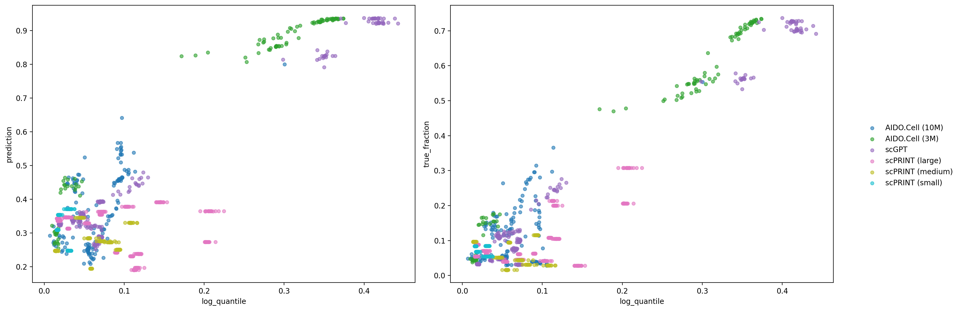
The scatterplots confirm that cross-model coherence and mechanistic enrichment are correlated: the layers where models converge on shared attention pairs are also those most enriched for reported interactions and high GNN scores. This suggests that cross-model agreement is not just a reproducibility check but an interpretable signal, identifying the layers and models most likely to capture genuine regulatory structure rather than architecture-specific noise.

Summary and future directions

This post extended the layer-wise attention analysis from Part 1 into two new dimensions: cross-model consistency and grounding in molecular interaction networks. Using a shared gene vocabulary across four model families and seven variants, I showed that intermediate layers of scGPT, AIDO.Cell (3M), and scPRINT (large) converge on overlapping sets of high-attention gene pairs despite differences in architecture, training data, vocabulary, and scale. Those same layers are also the most enriched for reported interactions in the Napistu Octopus network and for high GNN-predicted interaction scores, suggesting that cross-model coherence is a meaningful signal rather than architectural coincidence. The largest scPRINT model presents an instructive contrast: its attention patterns are mechanistically meaningful but biased toward cross-pathway interactions between dissimilar genes, an indication that it is precisely extracting the regulatory mechanisms that shape pathway crosstalk.

This framework opens several practical directions:

• Model selection and layer identification: cross-model coherence and interaction enrichment together provide a principled basis for identifying which model and which layers to use for a given downstream task, without requiring labeled data.
• Gene network inference: high-confidence attention pairs, particularly those consistently recovered across models and enriched for known interactions, can be used to construct cell-type-specific regulatory networks that go beyond co-expression.
• Model evaluation: the vocabulary-aligned comparison framework built here enables systematic benchmarking of new foundation models as they are released, assessing whether architectural or training innovations translate into improved mechanistic signals.

The deeper ambition behind this work is to bridge foundation model representations and actionable molecular biology. Attention patterns that are consistent across models and enriched for known regulatory interactions are not only interpretability curiosities; they are also candidate regulatory edges that can be prioritized for experimental follow-up. Beyond describing biology, a model that reliably attends to the edges of a signaling pathway in a disease-relevant cell type is generating hypotheses about which molecular interactions to perturb and which perturbations are most likely to shift cellular state in a desired direction. That is the translation from virtual cell to actionable intervention, and closing that gap is the goal this series is building toward.