Decoding Virtual Cell Foundation Models I: Architecture and Layer-wise Attention

Foundation models trained on large corpuses of single-cell RNA-seq data have emerged as one of the most promising frontier technologies in biotech. These models embed cells’ expression in a latent space, and then use a transformer architecture to attend to expression embeddings, learning functional coexpression patterns, which can be used to predict diverse properties such as cell type or denoised expression.

These models are built on massive datasets provided by Chan-Zuckerberg Initiative (CZI), Arc Institute, Tahoe Therapeutics and others (CellxGene, Tahoe 100M, Arc/BioHub/Tahoe announced collaboration). Emerging datasets bring additional cellular contexts, making more predictions in-distribution rather than out-of-distribution, and causal grounding with genetic perturbations provides the potential to move beyond coexpression. This causal signal is now being fruitfully mined with impressive results by Altos lab’s Cleopatra model in the Arc Institute’s 2025 Virtual Cell Challenge.

Foundation models themselves are continually evolving as academic and industry groups experiment with model architectures, inductive biases, new tasks, etc. There is a diverse array of models available through platforms like CZI models and NVIDIA BioNeMo which can be applied to single-cell RNAseq, sequences, analysis and structural prediction.

The excitement for foundation models and their evolution into multi-scale multi-modal Virtual Cell models is palpable; they form a cornerstone in the CZI’s aspirational goal to “cure, prevent, or manage all diseases by the end of this century.” (Incidentally, this would require stopping biological aging!)

A clear architecture for this ambition is nicely stated in “How to build the virtual cell with artificial intelligence: Priorities and opportunities”. In this paper, the authors highlight how universal representations of biology could be created at the level of molecules, cells, and multicellular interactions, and different data streams could feed into virtual cell models at an appropriate level. This provides the potential for both forward and reverse engineering biology — predicting how a DNA variant impacts tissue physiology, while also enabling us to backtrack from tissue pathophysiology to dysregulated molecular circuits (and drug targets!)

These universal representations can be supported with synthetic instruments to make diverse predictions, and also with decoders to map a virtual cell’s state back to human-interpretable, semantically-meaningful biology.

Here, I will lay the groundwork for decoding the attention mechanisms of four scRNAseq-based foundation models. Specifically, I will:

1. Provide an overview of single-cell foundation models, introducing abstractions which enable generalization.
2. Extract expression-contextualized gene embeddings and attention weights from scGPT, scFoundation, scPRINT, and AIDO.Cell using model-agnostic data structures.
3. Compare the geometry of the residual stream across layers within each model to assess how the organization of gene representation space evolves with depth.
4. Compare attention patterns across layers within each model to identify when the model has converged on stable gene-gene relationships.

In Part two, I’ll ground these attention patterns by benchmarking their consistency with reported interactions in Napistu’s 8-source Octopus network and their graph neural network (GNN) representations as a vertex embedding and interaction scoring model. There is a lot of build-up to the final results, but I think the payoff is worth it; scFMs tend to learn attention patterns which are consistent across models and agree with reported molecular interactions.

What is a single-cell RNAseq foundation model?

Understanding what these models have learned requires looking inside the transformer rather than treating them as black-box cell encoders. This means examining how genes relate to one another within a layer and how those relationships evolve across layers.

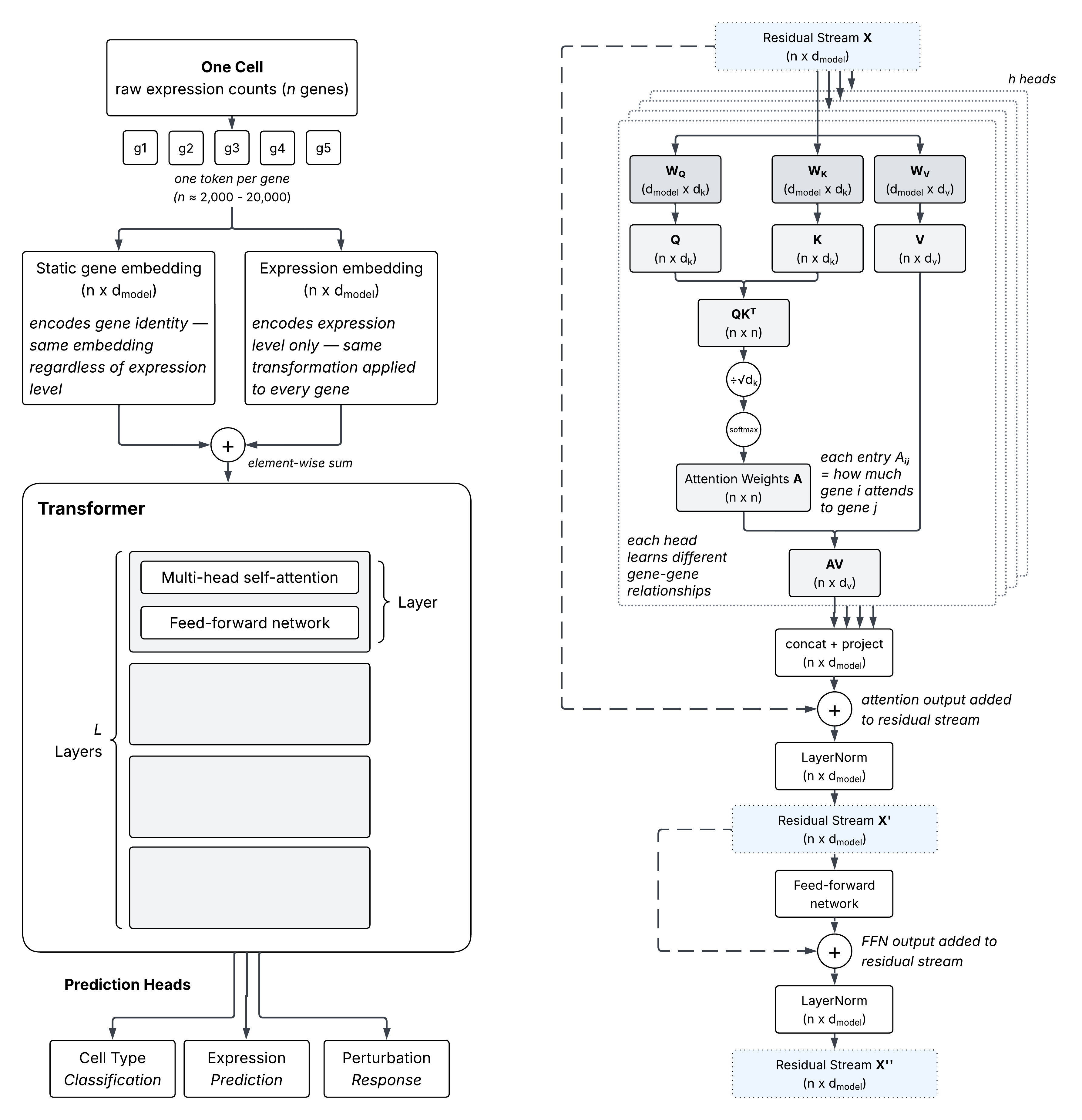
A gene expression foundation model takes a single cell as input and learns to represent it by processing thousands of genes simultaneously. Most models treat each expressed gene as a token (analogous to a word in a language model), combining its identity and expression level into a single vector before passing it into the transformer.

The transformer processes these gene tokens through multiple layers, each consisting of two operations applied in sequence. The attention sublayer lets every gene integrate information from all other genes, weighting contributions by relevance — the resulting $n \times n$ attention weight matrix $A$ has a direct interpretation, where entry $A_{ij}$ reflects how much gene $i$ attends to gene $j$ in that layer. The feed-forward sublayer then transforms each gene’s representation independently. Both operations write their outputs additively back to a shared residual stream: a gene-by-embedding matrix that persists across the full forward pass, with each sublayer reading from it and updating it in place. Early layers capture coarse expression structure; deeper layers accumulate biological context across the full transcriptional state of the cell.

The figure below shows the full architecture alongside a detailed view of how a single transformer layer operates — from the query ($Q$), key ($K$), and value ($V$) projections through the gene-gene attention weights to the feed-forward update.

The most common pretraining objective for bag-of-genes models is masked expression reconstruction; a random subset of gene expression values are zeroed out, and the model must predict the original values using only the remaining genes as context. This forces the model to learn co-expression relationships — to recover a masked gene’s expression, it must attend to genes that are co-regulated with it.

Not all foundation models fit neatly into this framework. Some, like Geneformer, use a ranked gene sequence rather than a bag of genes, ordering tokens by expression level rather than presenting them all simultaneously. Others, like UCE, sample gene tokens proportional to expression count, allowing the same gene to appear multiple times. These architectural choices affect what the model learns and how its representations can be interpreted.

The table below summarizes how eight prominent foundation models instantiate this general framework, highlighting the key architectural choices that determine what each model attends to and what it learns.

Processing four foundation models with a common workflow

Each foundation model arrives with its own ecosystem: private Python dependencies, bespoke preprocessing pipelines, and idiosyncratic gene vocabularies. Rather than focusing on a single model, where the generality of findings would be difficult to establish, I set up a common workflow to process and compare four bag-of-genes models. This required a two-environment pattern. A model-specific ETL environment handles loading, preprocessing, and the forward pass for each model, extracting three things:

1. Model weights — the $Q$, $K$, and $V$ projection matrices for each transformer layer, with heads concatenated along the embedding dimension
2. Model metadata — name, variant, layer count, head count, and parameter count
3. Residual streams — the gene-by-embedding matrix at each layer, averaged within cell-type clusters across individual cell forward passes. For practical reasons, I only processed a limited number of cells-per-category for most models, generally 50 or 100 cells.

A shared analysis environment then loads these standardized outputs using Napistu-Torch, enabling equivalent comparisons across all four models.

When a cell’s expression profile is passed through the model, the transformer builds a residual stream for that cell — a sequence of gene-by-embedding snapshots, one per layer, where each layer’s attention and feed-forward updates accumulate biological context. Rather than analyzing individual cells, I run forward passes on individual cells and average the residual stream within cell-type clusters at each layer. A cluster’s average embedding remains close to its individual members in latent space, so the aggregation is faithful, and cell-type resolution is the natural unit for mechanistic interpretation; we want to understand is which regulatory circuits are active in a given cell type, not which are active in a single noisy observation.

The dataset used throughout this analysis comes from Eftimiou et al. 2025, a single-nucleus RNA-seq atlas of human white adipose tissue, obtained through CellxGene. White adipose tissue is a useful testbed for this kind of analysis: it contains a diverse mixture of well-separated cell types — from metabolism-focused adipocytes and fibroadipogenic progenitors to immune and endothelial populations — with expression structure that organizes cleanly by cell type and no obvious major technical confounders. That diversity is useful precisely because we might expect quite different gene regulatory programs to be active across cell types, giving the models’ attention patterns something meaningful to differentiate.

Getting started

Reproducing this analysis

Unlike most posts on this site, this analysis cannot be reproduced by downloading a single artifact — the residual streams total ~25 GB, making them impractical to host publicly. To follow along on your own machine, you’ll need to run the model-specific ETL notebooks to generate the residual streams locally, then set up the analysis environment below.

1. For model-specific processing refer to foundation model ETL. Each notebook describes its own environment setup and uses napistu-torch for extracting weights and residual streams.

2. Install uv (or use pip if preferred) and set up the analysis environment:

uv venv --python 3.11
source .venv/bin/activate
# Core dependencies
uv pip install torch==2.8.0
uv pip install "napistu-torch==0.4.0"
# if you'd like to render the notebook, you'll need to install these additional dependencies
uv pip install seaborn ipykernel nbformat nbclient umap-learn
uv pip install git+https://github.com/shackett/shackett-utils.git
python -m ipykernel install --user --name=blog-staging

1. Download the sc_foundation_model_overview.qmd notebook (or copy and paste the relevant code blocks).

2. Configure PROJECT_DIR and other paths in the env_setup code block to point to your local directories.

Configuration and imports

# standard library
import logging
import re
from pathlib import Path
from typing import Dict, List, Tuple

# 3rd party
import numpy as np
import pandas as pd
import matplotlib.pyplot as plt
from matplotlib.colors import LinearSegmentedColormap
import seaborn as sns

# Napistu
from napistu.utils import load_pickle, save_pickle

# Napistu-Torch
from napistu_torch.foundation_models.attention_patterns import LayerwiseAttentionInputs
from napistu_torch.foundation_models.constants import (
    COMPARE_EMBEDDINGS_COMPARISONS,
    FOUNDATION_MODEL_NAMES,
    MODEL_NICE_NAMES,
)
from napistu_torch.foundation_models.foundation_models import (
    FoundationModel,
    FoundationModelStore,
    FoundationModels,
    _get_disk_name,
)
from napistu_torch.foundation_models.gene_embeddings import GeneEmbeddingsSet
from napistu_torch.visualization.heatmaps import plot_heatmap
from shackett_utils.blog.html_utils import display_tabulator

logging.basicConfig(level=logging.INFO, format='%(levelname)s:%(name)s:%(message)s')
logger = logging.getLogger(__name__)

# paths
PROJECT_DIR = Path("~/Desktop/DATA/sc_foundation_models").expanduser()
CACHE_DIR = PROJECT_DIR / "cache"
MODEL_OUTPUTS_DIR = PROJECT_DIR / "model_outputs"  # where extracted foundation model weights live

# settings
IGNORE_CATEGORIES_WITH = ["unknown"]
IGNORED_MODELS = ["AIDOCell_aido_cell_100m"]
EMBEDDING_DATASET = "efthymiou2025"  # adipose tissue dataset from Eftimiou et al. 2025
BY_ABSOLUTE_VALUE = False  # select top attention pairs by most positive value (not absolute)
TOP_K = 10000             # primary K for rank-agreement heatmaps
K_SENSITIVITY_VALUES = [1000, 5000, 10000, 50000]  # K values for robustness check; must include TOP_K
IGNORE_SELF_ATTENTION = True
OVERWRITE = False
VERBOSE = False

# Diverging palettes
# steelblue1 #63B8FF, yellow #FFFF00 (R ``yellow``), black #000000.
bwy = LinearSegmentedColormap.from_list(
    "steelblue1_black_yellow",
    ["#63B8FF", "#000000", "#FFFF00"],
)

# blue #1D4A7A, white #F0EDE8, red #C01D2E
bwr = LinearSegmentedColormap.from_list(
    "red_white_blue",
    ["#1D4A7A", "#F0EDE8", "#C01D2E"],  # flip: blue=low, red=high
)

def to_filename(s: str) -> str:
    s = re.sub(r"[^\w\s-]", "", s)
    s = re.sub(r"\s+", "_", s)
    return s.strip("-_")

def get_model_names(
    include_scgpt: bool = True,
    include_scfoundation: bool = True,
    ignored_models: List[str] | None = None,
) -> List[str]:
    ignored = ignored_models or []
    full_names = [
        _get_disk_name(model_name, model_variant)
        for model_name, model_variant in MODEL_NICE_NAMES
        if include_scgpt or model_name != FOUNDATION_MODEL_NAMES.SCGPT
        if include_scfoundation or model_name != FOUNDATION_MODEL_NAMES.SCFOUNDATION
    ]
    if ignored:
        invalid = [name for name in ignored if name not in full_names]
        if invalid:
            logger.warning(f"Ignored models not found in known model names: {invalid}")
        full_names = [name for name in full_names if name not in ignored]
    return full_names

def n_genes_in_dataset_embedding_summary(
    disk_name_or_model: str | FoundationModel,
    model_outputs_dir: Path,
    embedding_dataset: str,
    ignore_categories_with: List[str],
) -> int | str:
    if isinstance(disk_name_or_model, str):
        model = FoundationModel.load(Path(model_outputs_dir) / disk_name_or_model)
        disk_tag = disk_name_or_model
    else:
        model = disk_name_or_model
        disk_tag = model.disk_name

    categories = sorted([
        category
        for category in model.store.list_categories(embedding_dataset)
        if not any(substring in category for substring in ignore_categories_with)
    ])
    if not categories:
        raise ValueError(f"No categories for model {disk_tag!r} in dataset {embedding_dataset!r}")

    counts: List[int] = []
    for category in categories:
        residuals = model.load_category_residuals(embedding_dataset, category)
        counts.append(next(iter(residuals.values())).n_genes)

    uniq = sorted(set(counts))
    if len(uniq) == 1:
        return uniq[0]
    return f"{min(counts)}\u2013{max(counts)}"

def get_model_label_maps(model_metadata_summary: pd.DataFrame) -> Tuple[dict, dict]:
    model_type_map = model_metadata_summary.set_index("model")["model type"].to_dict()
    model_variant_map = model_metadata_summary.set_index("model")["model variant"].to_dict()
    return model_type_map, model_variant_map

def get_model_categories(
    model_name: str,
    model_outputs_dir: Path,
    embedding_dataset: str,
    ignore_categories_with: List[str],
) -> List[str]:
    store = FoundationModelStore(Path(model_outputs_dir) / model_name)
    return sorted([
        category
        for category in store.list_categories(embedding_dataset)
        if not any(substring in category for substring in ignore_categories_with)
    ])

def get_cache_path(model_name: str, category: str, cache_dir: Path) -> Path:
    return cache_dir / f"within_model_{to_filename(model_name)}_{to_filename(category)}.pkl"

def get_model_comparison_metadata(
    model_outputs_dir: Path,
    embedding_dataset: str,
    ignore_categories_with: List[str],
    ignored_models: List[str],
) -> Dict:
    model_names = get_model_names(ignored_models=ignored_models)
    models = FoundationModels.load_multiple(model_outputs_dir, model_names, verbose=False)

    model_metadata_summary = models.get_summary().rename(columns={
        "full_name": "model",
        "model": "model type",
        "variant": "model variant",
        "embed_dim": "# dim",
        "n_layers": "# layers",
        "n_heads": "# heads",
        "parameter_count": "# parameters",
    })

    model_metadata_summary["# genes"] = [
        n_genes_in_dataset_embedding_summary(
            model,
            model_outputs_dir=model_outputs_dir,
            embedding_dataset=embedding_dataset,
            ignore_categories_with=ignore_categories_with,
        )
        for model in models.models
    ]

    disk_name_by_full_name = {
        model.full_name: model.disk_name for model in models.models
    }

    return {
        "model_order": models.model_names,
        "disk_name_by_full_name": disk_name_by_full_name,
        "model_metadata_summary": model_metadata_summary,
    }

def model_facet_mosaic_layout(n: int) -> Tuple[List[List[str]], List[float]]:
    if n < 1:
        raise ValueError("n must be >= 1")
    n_cols = max(1, int(np.ceil(n / 2)))
    n_rows = int(np.ceil(n / n_cols))
    layout: List[List[str]] = []
    k = 0
    for _ in range(n_rows):
        row: List[str] = []
        for _col in range(n_cols):
            row.append(str(k) if k < n else ".")
            k += 1
        layout.append(row)
    width_ratios = [1.0] * n_cols
    return layout, width_ratios

def residual_corr_to_matrix(residual_corr: Dict[str, float], n_layers: int) -> pd.DataFrame:
    mat = np.full((n_layers, n_layers), np.nan)
    np.fill_diagonal(mat, 1.0)
    for key, rho in residual_corr.items():
        indices = [int(x) for x in re.findall(r"(?<=layer_)\d+", key)]
        if len(indices) == 2:
            i, j = indices
            mat[i, j] = rho
            mat[j, i] = rho
    return pd.DataFrame(mat)

def compute_within_model_layer_comparisons(
    model: FoundationModel,
    dataset_name: str,
    category: str,
    top_k: int,
    k_sensitivity_values: List[int],
    by_absolute_value: bool = False,
    ignore_self_attention: bool = True,
    verbose: bool = False,
) -> Dict:
    if top_k not in k_sensitivity_values:
        raise ValueError(f"top_k={top_k} must be in k_sensitivity_values={k_sensitivity_values}")

    residuals = model.load_category_residuals(dataset_name, category)
    lwa = LayerwiseAttentionInputs(residual_stream_embeddings=residuals, foundation_model=model)

    layer_rank_by_k = {}
    for k in k_sensitivity_values:
        layer_corr_k, layer_rank_k = lwa.compare_layer_attention_consistency(
            top_k=k,
            by_absolute_value=by_absolute_value,
            ignore_self_attention=ignore_self_attention,
            verbose=verbose,
        )
        layer_rank_by_k[k] = layer_rank_k
        if k == top_k:
            layer_corr = layer_corr_k
            layer_rank = layer_rank_k

    embedding_set = GeneEmbeddingsSet.from_gene_embeddings(
        [residuals[i] for i in sorted(residuals.keys())]
    )
    residual_stream_layer_corr = embedding_set.compare_embeddings()

    return {
        COMPARE_EMBEDDINGS_COMPARISONS.MODEL_LAYER_CORRELATIONS: layer_corr,
        COMPARE_EMBEDDINGS_COMPARISONS.MODEL_LAYER_RANK_AGREEMENT: layer_rank,
        "layer_rank_by_k": layer_rank_by_k,
        "residual_stream_layer_correlations": residual_stream_layer_corr,
    }

def aggregate_model_categories(
    model_name: str,
    k_sensitivity_values: List[int],
    cache_dir: Path,
    model_outputs_dir: Path,
    embedding_dataset: str,
    ignore_categories_with: List[str],
) -> Dict:
    categories = get_model_categories(
        model_name,
        model_outputs_dir=model_outputs_dir,
        embedding_dataset=embedding_dataset,
        ignore_categories_with=ignore_categories_with,
    )

    cat_layer_corrs: List[np.ndarray] = []
    cat_rank_dfs: List[pd.DataFrame] = []
    cat_rank_by_k: Dict[int, List[pd.DataFrame]] = {k: [] for k in k_sensitivity_values}
    cat_residual_pairs: Dict[str, List[float]] = {}

    for category in categories:
        data = load_pickle(get_cache_path(model_name, category, cache_dir=cache_dir))
        cat_layer_corrs.append(data[COMPARE_EMBEDDINGS_COMPARISONS.MODEL_LAYER_CORRELATIONS])
        cat_rank_dfs.append(data[COMPARE_EMBEDDINGS_COMPARISONS.MODEL_LAYER_RANK_AGREEMENT])
        for k in k_sensitivity_values:
            cat_rank_by_k[k].append(data["layer_rank_by_k"][k])
        for pair, rho in data["residual_stream_layer_correlations"].items():
            cat_residual_pairs.setdefault(pair, []).append(rho)

    return {
        COMPARE_EMBEDDINGS_COMPARISONS.MODEL_LAYER_CORRELATIONS: np.median(cat_layer_corrs, axis=0),
        COMPARE_EMBEDDINGS_COMPARISONS.MODEL_LAYER_RANK_AGREEMENT: (
            pd.concat(cat_rank_dfs)
            .groupby(["query_layer", "eval_layer"])["median_quantile"]
            .median()
            .reset_index()
        ),
        "layer_rank_by_k": {
            k: (
                pd.concat(dfs)
                .groupby(["query_layer", "eval_layer"])["median_quantile"]
                .median()
                .reset_index()
            )
            for k, dfs in cat_rank_by_k.items()
        },
        "residual_stream_layer_correlations": {
            pair: float(np.median(rhos)) for pair, rhos in cat_residual_pairs.items()
        },
    }

def plot_rank_agreement_by_layer(
    layer_rank_by_k,
    K_values,
    model_order,
    model_metadata_summary,
    figsize=(14, 4),
    group_gap=2,
    reference_value=0.5,
):
    k_colors = ["#E63946", "#2196F3", "#FF9800", "#4CAF50"]
    color_map = dict(zip(sorted(K_values), k_colors))

    model_type_map, model_variant_map = get_model_label_maps(model_metadata_summary)
    fig, ax = plt.subplots(figsize=figsize)

    x_pos_map = {}
    current_x = 0
    model_label_positions = {}

    for model in model_order:
        sample_k = sorted(K_values)[0]
        rank_df = layer_rank_by_k[model][sample_k]
        consecutive = rank_df[rank_df["eval_layer"] == rank_df["query_layer"] + 1]
        query_layers = sorted(consecutive["query_layer"].unique())

        model_start = current_x
        for layer in query_layers:
            x_pos_map[(model, layer)] = current_x
            current_x += 1
        model_label_positions[model] = (model_start + current_x - 1) / 2
        current_x += group_gap

    for model in model_order:
        for k in sorted(K_values):
            rank_df = layer_rank_by_k[model][k]
            consecutive = (
                rank_df[rank_df["eval_layer"] == rank_df["query_layer"] + 1]
                .sort_values("query_layer")
                .assign(median_quantile=lambda x: 1 - x["median_quantile"])
            )
            xs = [
                x_pos_map[(model, ql)]
                for ql in consecutive["query_layer"]
                if (model, ql) in x_pos_map
            ]
            ys = [
                row["median_quantile"]
                for _, row in consecutive.iterrows()
                if (model, row["query_layer"]) in x_pos_map
            ]
            ax.plot(
                xs,
                ys,
                marker="o",
                markersize=4,
                color=color_map[k],
                label=f"K = {k:,}",
                linewidth=1.5,
            )

    all_xticks = []
    all_xlabels = []
    for model in model_order:
        sample_k = sorted(K_values)[0]
        rank_df = layer_rank_by_k[model][sample_k]
        consecutive = rank_df[rank_df["eval_layer"] == rank_df["query_layer"] + 1]
        for layer in sorted(consecutive["query_layer"].unique()):
            if (model, layer) in x_pos_map:
                all_xticks.append(x_pos_map[(model, layer)])
                all_xlabels.append(str(layer))

    ax.set_xticks(all_xticks)
    ax.set_xticklabels(all_xlabels, fontsize=7)
    ax.axhline(reference_value, color="gray", linestyle=":", linewidth=1.5, zorder=0)
    ax.set_xlabel("Layer")
    ax.set_ylabel("Median quantile of top-K pairs\nin next layer")
    ax.set_ylim(0, 1)
    ax.grid(True, alpha=0.3, axis="y")
    plt.tight_layout()

    y_max = ax.get_ylim()[1]
    y_type = y_max * 1.12
    y_variant = y_max * 1.04
    seen_types = {}

    for model, x_center in model_label_positions.items():
        model_type = model_type_map.get(model, model)
        variant = model_variant_map.get(model)
        if model_type not in seen_types:
            seen_types[model_type] = []
        seen_types[model_type].append(x_center)
        if pd.notna(variant):
            ax.text(
                x_center,
                y_variant,
                variant,
                ha="center",
                va="bottom",
                fontsize=8,
                color="#555555",
            )

    for model_type, positions in seen_types.items():
        ax.text(
            np.mean(positions),
            y_type,
            model_type,
            ha="center",
            va="bottom",
            fontsize=10,
            fontweight="bold",
        )

    handles = [
        plt.Line2D([0], [0], color=color_map[k], marker="o", label=f"K = {k:,}")
        for k in sorted(K_values)
    ]
    ax.legend(
        handles=handles,
        bbox_to_anchor=(1.01, 0.5),
        loc="center left",
        frameon=False,
        fontsize=9,
    )

    plt.suptitle(
        "Consecutive-layer rank consistency is stable across K",
        fontweight="bold",
        fontsize=11,
        y=1.15,
    )

    return fig, ax

Building the cache

For each model and cell-type cluster, I precomputed within-model layer comparisons and saved them to disk.

model_names = get_model_names(ignored_models=IGNORED_MODELS)

for model_name in model_names:
    model = FoundationModel.load(MODEL_OUTPUTS_DIR / model_name, verbose=VERBOSE)
    categories = get_model_categories(
        model_name,
        model_outputs_dir=MODEL_OUTPUTS_DIR,
        embedding_dataset=EMBEDDING_DATASET,
        ignore_categories_with=IGNORE_CATEGORIES_WITH,
    )

    for category in categories:
        cache_path = get_cache_path(model_name, category, cache_dir=CACHE_DIR)
        if cache_path.is_file() and not OVERWRITE:
            if VERBOSE:
                logger.info(f"Skipping {model_name}: {category}, cache exists")
            continue

        logger.info(f"Running {model_name}: {category}")

        result = compute_within_model_layer_comparisons(
            model=model,
            dataset_name=EMBEDDING_DATASET,
            category=category,
            top_k=TOP_K,
            k_sensitivity_values=K_SENSITIVITY_VALUES,
            by_absolute_value=BY_ABSOLUTE_VALUE,
            ignore_self_attention=IGNORE_SELF_ATTENTION,
            verbose=VERBOSE,
        )
        save_pickle(cache_path, result)

Loading and aggregating

Cached results are loaded and aggregated across cell-type clusters for each model, producing four layer-indexed outputs used in the analyses below.

model_comparison_metadata = get_model_comparison_metadata(
    model_outputs_dir=MODEL_OUTPUTS_DIR,
    embedding_dataset=EMBEDDING_DATASET,
    ignore_categories_with=IGNORE_CATEGORIES_WITH,
    ignored_models=IGNORED_MODELS,
)
model_order = model_comparison_metadata["model_order"]
disk_name_by_full_name = model_comparison_metadata["disk_name_by_full_name"]
model_metadata_summary = model_comparison_metadata["model_metadata_summary"]
n_layers_map = model_metadata_summary.set_index("model")["# layers"].to_dict()

aggregated = {
    model_name: aggregate_model_categories(
        disk_name_by_full_name[model_name],
        K_SENSITIVITY_VALUES,
        cache_dir=CACHE_DIR,
        model_outputs_dir=MODEL_OUTPUTS_DIR,
        embedding_dataset=EMBEDDING_DATASET,
        ignore_categories_with=IGNORE_CATEGORIES_WITH,
    )
    for model_name in model_order
}

residual_stream_layer_correlations: Dict[str, Dict] = {m: v["residual_stream_layer_correlations"] for m, v in aggregated.items()}
model_layer_correlations: Dict[str, np.ndarray] = {m: v[COMPARE_EMBEDDINGS_COMPARISONS.MODEL_LAYER_CORRELATIONS] for m, v in aggregated.items()}
model_layer_rank_agreement: Dict[str, pd.DataFrame] = {m: v[COMPARE_EMBEDDINGS_COMPARISONS.MODEL_LAYER_RANK_AGREEMENT] for m, v in aggregated.items()}
layer_rank_by_k: Dict[str, Dict[int, pd.DataFrame]] = {m: v["layer_rank_by_k"] for m, v in aggregated.items()}

How foundation models build gene and interaction representations

Four bag-of-genes model families are represented here across seven variants. They span nearly two orders of magnitude in parameter count, from the 393K-parameter AIDO.Cell (3M) to the 28M-parameter scFoundation. They also differ substantially in gene vocabulary: scGPT processes only 1,200 genes per cell following its preprocessing, while scPRINT and AIDO.Cell embed 18-19K. scPRINT’s three size variants make it particularly useful for examining how scale affects the representations and attention patterns analyzed below.

display_tabulator(
    model_metadata_summary,
    layout="fitDataTable",
    include_index=False,
)

One architectural distinction visible in the table is scFoundation’s variable gene vocabulary. Rather than operating on a fixed token set, scFoundation restricts its forward pass to genes with at least one count, so individual cells have distinct vocabularies. To create a cluster-level summary, I averaged the residual stream across non-NaN values for each gene and reported only genes detected in at least two cells; the number of genes represented consequently varies across cell categories, ranging from roughly five to ten thousand in this dataset.

Layer-wise reorganization of gene representation space

To track how each model’s internal representations evolve with depth, I computed the gene-gene cosine similarity matrix at each layer of the residual stream — a snapshot of which genes are near each other in representation space at that layer. I then measured how similar those snapshots are across layers using Spearman ρ, correlating the full similarity matrices pairwise. This approach, sometimes called representational similarity analysis, has the useful property of being invariant to embedding dimension, so comparisons are valid both within and across models.

The resulting matrices are shown below. A value near 1 between layers $i$ and $j$ means the geometry of gene representation space is nearly identical at those two depths; a lower value means the model has substantially reorganized which genes are near which other genes.

_layout, width_ratios = model_facet_mosaic_layout(len(model_order))
fig, axd = plt.subplot_mosaic(
    _layout,
    figsize=(20, 13),
    gridspec_kw={"width_ratios": width_ratios},
)

for idx, model_name in enumerate(model_order):
    n_layers = int(n_layers_map[model_name])
    data = residual_corr_to_matrix(residual_stream_layer_correlations[model_name], n_layers)
    annot_size = 15 - 2 * np.sqrt(n_layers)

    plot_heatmap(
        data,
        row_labels=range(n_layers),
        title=model_name,
        cbar=False,
        fmt='.2f',
        vmax=1,
        vmin=-1,
        cbar_label='Spearman ρ',
        cmap=bwy,
        mask_upper_triangle=True,
        square=True,
        title_size=22,
        annot_size=annot_size,
        title_fontstyle="italic",
        ax=axd[str(idx)],
    )

plt.suptitle(
    "Within-model residual stream layer correlations\n"
    "(Spearman ρ of gene-gene cosine similarity across layers)",
    fontsize=24, fontweight="bold",
)
plt.tight_layout(rect=[0, 0, 1, 0.97])
plt.show()

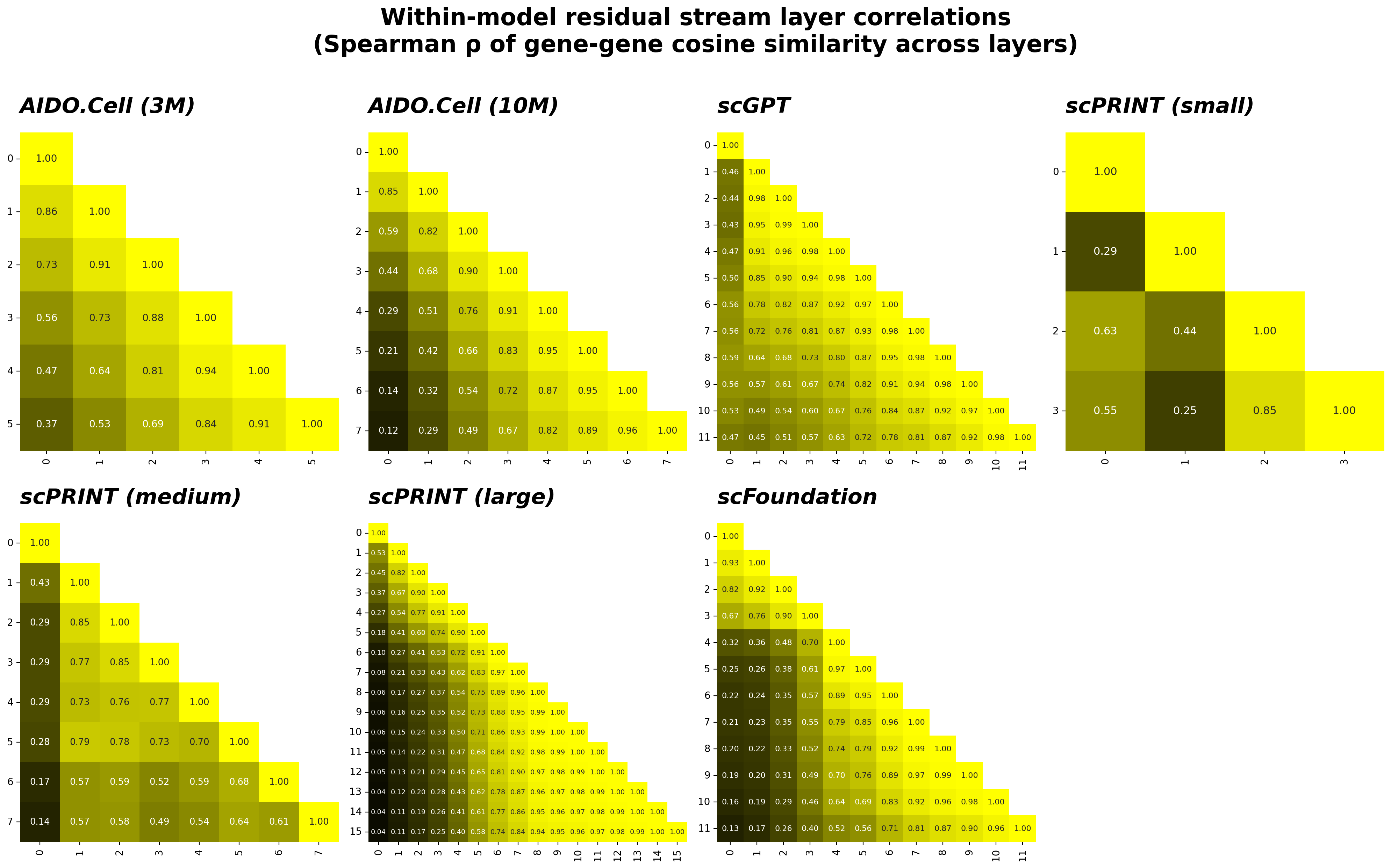
The clearest pattern across all models is that the residual stream is progressively evolving — adjacent layers are highly correlated, but early and late layers are not, reflecting the cumulative effect of each attention and FFN update writing into the stream. This is expected: because each sublayer adds to rather than replaces the stream, the geometry drifts progressively rather than jumping.

The stable residual stream in scPRINT large is most likely a signature of undertraining relative to its architectural depth. Compared to scPRINT medium — which shows the expected progressive decorrelation across 8 layers — the large model doubles the depth to 16 layers while keeping the head count fixed at 4. With only 4 attention heads writing into a 512-dimensional stream, later layers may not have received sufficient gradient signal to learn updates that are meaningfully distinct from their predecessors. The result is a stack of near-identity transforms: each sublayer nominally adds to the residual stream, but the additions are small and geometrically consistent enough that the stream barely drifts. This is a common failure mode when architectural expressivity outruns the training budget — the model’s depth becomes effectively nominal rather than functional, and the residual stream reflects early-layer geometry throughout.

Layer-wise attention routing and gene-pair selection

The residual stream analyses above show smooth, progressive drift across layers — a natural consequence of each sublayer adding to rather than replacing the stream. Attention patterns do not inherit this property. Each layer’s weights are determined independently, so the patterns that emerge layer-to-layer could in principle reinforce one another, oppose one another, or focus on largely orthogonal aspects of gene-gene relationships.

The attention weights at each layer describe which gene pairs the model is actively drawing on when building each gene’s contextualized representation. Each layer produces an $N×N$ matrix of directed pair weights, where rows index query genes and columns index key genes — entry ($i$,$j$) reflects how strongly gene $i$ draws on gene $j$ when building its contextualized representation. For a transcriptome-wide model with ~20K genes that is 400M entries per layer, the vast majority of which receive near-zero weight. The biologically informative signal is concentrated in the high-attention tail: the pairs where one gene is strongly drawing on another to contextualize itself. Selecting the top-K pairs focuses the analysis on this sparse, high-signal subset and keeps cross-layer comparisons tractable.

Spearman correlation across the union of top 10K attention pairs

For each layer, I extracted the top-K gene pairs by attention weight — where attention is computed as the head-averaged softmax of the scaled dot-product $Q K^\top / \sqrt{d_k}$ — and the union of these sets is taken across all layers. Each layer is then represented as a vector of weights over this shared index, and Spearman correlations are computed between all layer pairs.

_layout, width_ratios = model_facet_mosaic_layout(len(model_order))
fig, axd = plt.subplot_mosaic(
    _layout,
    figsize=(20, 13),
    gridspec_kw={"width_ratios": width_ratios},
)

for idx, model_name in enumerate(model_order):
    data = pd.DataFrame(model_layer_correlations[model_name])
    annot_size = 15 - 2 * np.sqrt(data.shape[0])

    plot_heatmap(
        data,
        row_labels=range(data.shape[0]),
        title=model_name,
        cbar=False,
        fmt='.2f',
        vmax=1,
        vmin=-1,
        cbar_label='Spearman ρ',
        cmap=bwy,
        mask_upper_triangle=True,
        square=True,
        title_size=22,
        annot_size=annot_size,
        title_fontstyle="italic",
        ax=axd[str(idx)],
    )

plt.suptitle(
    "Within-model layer × layer Spearman correlations using top attention pairs",
    fontsize=24, fontweight="bold",
)
plt.tight_layout(rect=[0, 0, 1, 0.98])
plt.show()

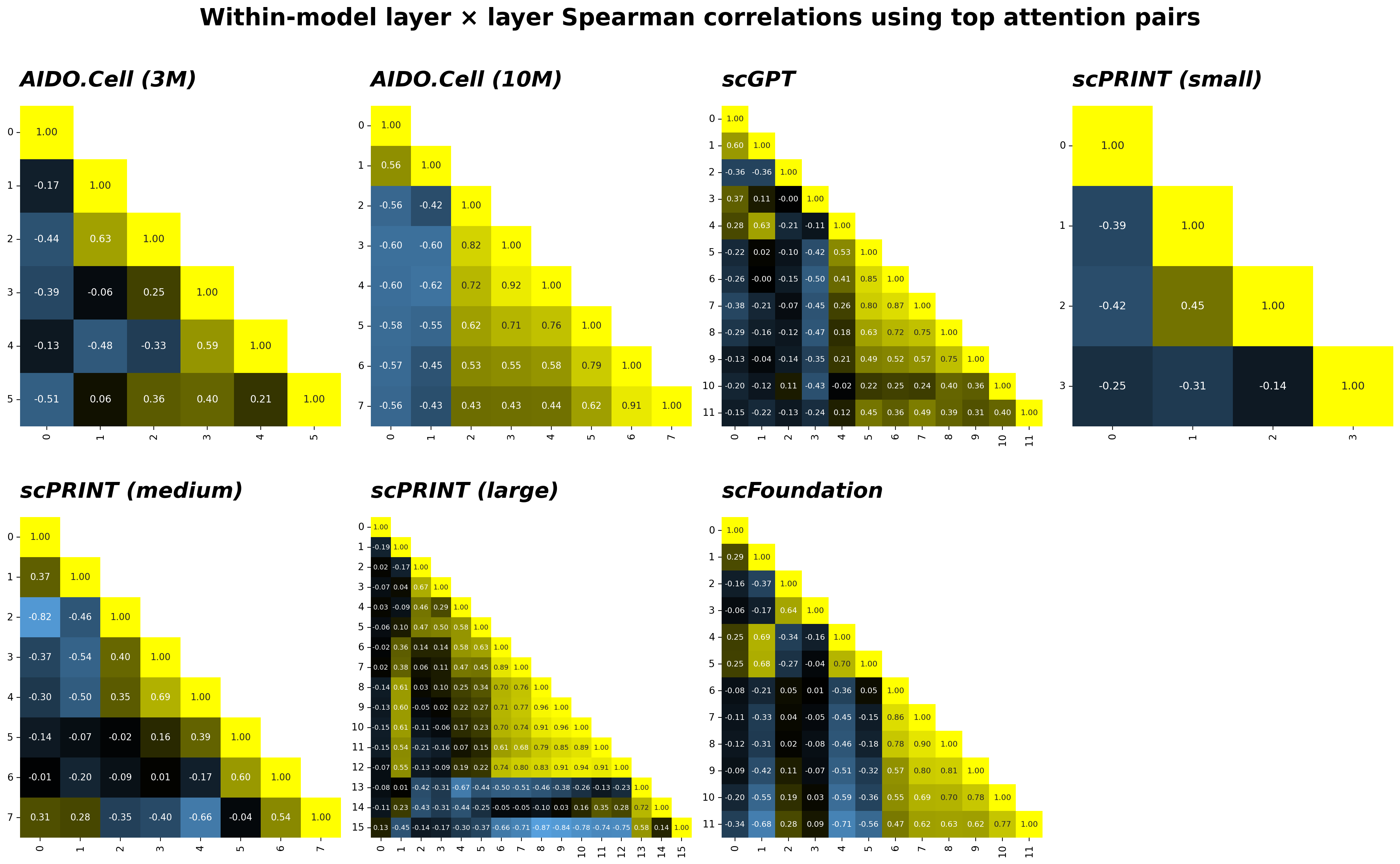
Across models, adjacent layers show moderate positive correlation but the relationship decays quickly with depth, and negative correlations between non-adjacent layers are common. This reflects genuine layer-wise specialization; different layers are routing attention to different gene pairs rather than reinforcing a single stable pattern.

Conditional attention quantiles to address winner’s curse

The cross-layer Spearman correlations above understate true coherence due to a winner’s curse artifact: selecting the top-K pairs from one layer means those pairs will tend to rank lower in other layers by regression to the mean alone, even when the underlying biology is shared. This inflates apparent divergence.

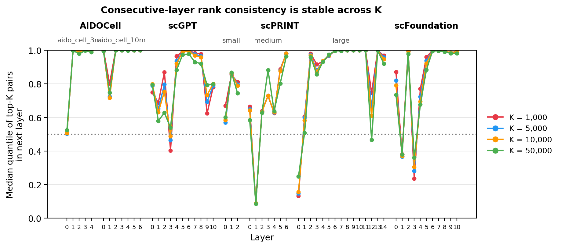
The rank-agreement metric addresses this directly; for a query layer, the top-K pairs are selected, and the median quantile of those pairs is evaluated in every other layer using that layer’s own attention distribution. If a second layer assigns most of the query layer’s top pairs to the upper tail of its own ranking, that is evidence of genuine cross-layer coherence rather than a selection artifact.

_layout, width_ratios = model_facet_mosaic_layout(len(model_order))
n_cols = len(_layout[0])
n_rows = len(_layout)
fig, axd = plt.subplot_mosaic(
    _layout,
    figsize=(20, 13),
    gridspec_kw={"width_ratios": width_ratios},
)

for idx, model_name in enumerate(model_order):

    conditional_quantiles = (
        model_layer_rank_agreement[model_name]
        # convert from rank quantiles (0 is strongest agreement) to ordinary quantiles (1 indicates the strongest agreement)
        .assign(median_quantile=lambda x: 1 - x["median_quantile"])
        .pivot_table(
            index="query_layer", columns="eval_layer", values="median_quantile", aggfunc="median"
        )
    )

    row, col = divmod(idx, n_cols)
    x_title = "Evaluation layer" if row == n_rows - 1 else None
    y_title = f"Top {TOP_K} layer" if col == 0 else None
    annot_size = 15 - 2 * np.sqrt(conditional_quantiles.shape[0])

    plot_heatmap(
        conditional_quantiles,
        row_labels=range(conditional_quantiles.shape[0]),
        title=model_name,
        xlabel=x_title,
        ylabel=y_title,
        cbar=False,
        cmap=bwr,
        fmt='.2f',
        vmax=1,
        vmin=0,
        mask_upper_triangle=False,
        square=True,
        title_size=22,
        axis_title_size=18,
        annot_size=annot_size,
        title_fontstyle="italic",
        ax=axd[str(idx)],
    )

plt.suptitle(
    "Median quantiles in an evaluation layer of the top K pairs in a query layer",
    fontsize=24, fontweight="bold",
)
plt.tight_layout(rect=[0, 0, 1, 0.98])
plt.show()

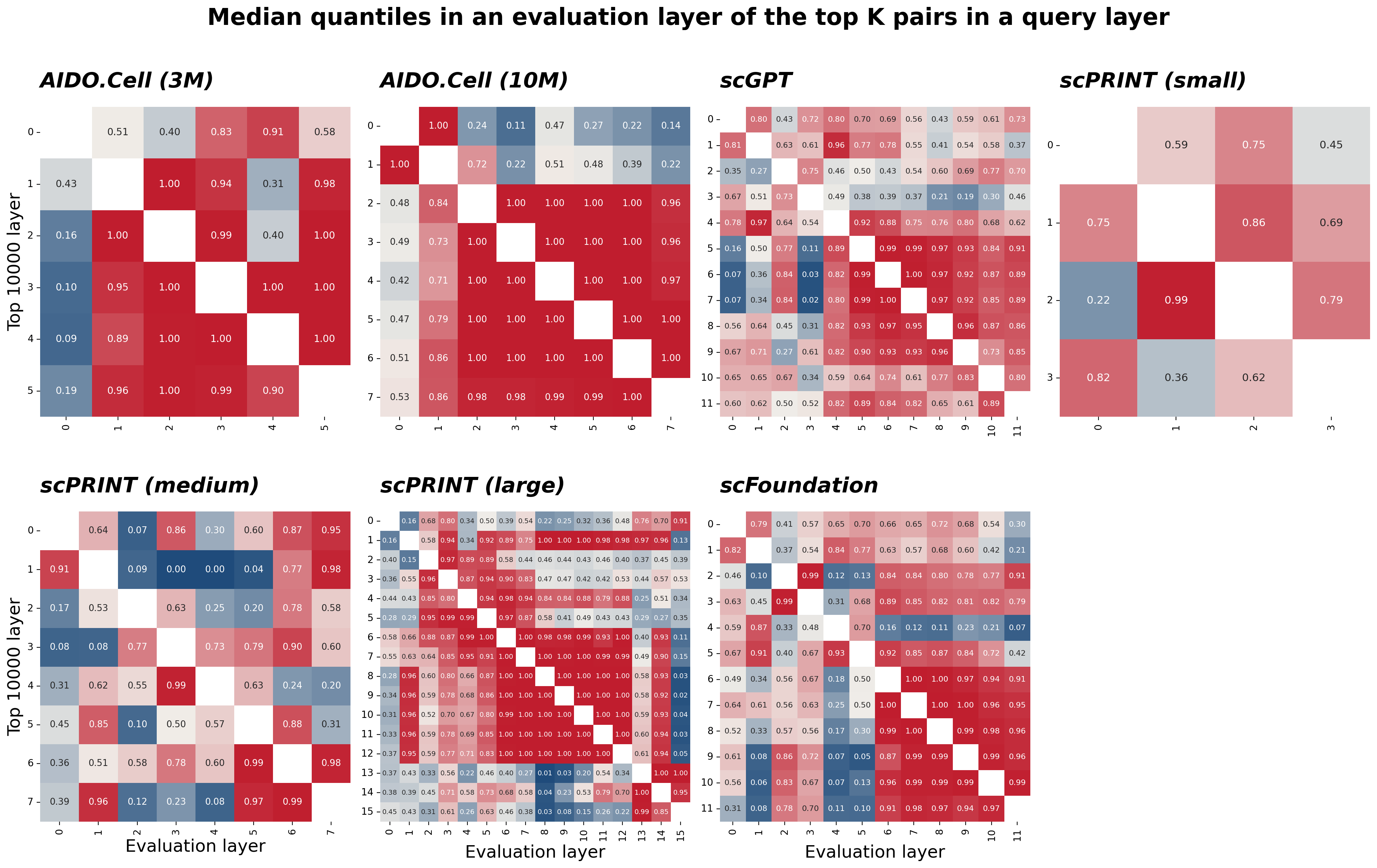
The rank-agreement matrices largely confirm the Spearman patterns: adjacent layers show strong agreement while early and late layers often strongly disagree. The directional metric adds resolution by separating the upper triangle (how well early-layer top pairs score when evaluated in late layers) from the lower triangle (how well late-layer top pairs score when evaluated in early layers). This asymmetry reveals that the anticorrelation between early and late layers reflects a directional canceling of early attention structure, which manifests in two ways:

• Suppression: the upper triangle is cold across most models — late layers actively down-rank the gene pairs that early layers prioritized, canceling the signal those early layers wrote into the residual stream.
• Catch-up: in AIDO.Cell (3M), scGPT, and scPRINT (medium), cold patches in the lower triangle reveal the mirror image — late layers specifically elevate pairs that early layers had most strongly suppressed, canceling out the early negative signal rather than the early positive signal.

Both are consistent with a picture where early layers perform a transient reorganization of the residual stream that is partially or fully reversed by later layers. This suggests that some early attention structure is useful for intermediate computation but not for the final cellular representation.

Robustness to choice of K

The patterns above — suppression, catch-up, and the transient reorganization picture — were all computed at a fixed K. A reasonable question is whether the choice of cutoff is driving the result or whether the signal is stable across a range of top-K thresholds.

Evaluating rank consistency across every pair of layers would produce $O(L^2)$ comparisons per model — useful for a full similarity matrix but hard to read across seven models simultaneously. Consecutive-layer pairs ($i \to i+1$) compress this into a single interpretable trajectory: how much the top-K pair rankings shift as representations pass through each successive layer.

The plot below applies this across K = 1,000 to 50,000. Each line shows the median quantile of the top-K gene pairs from layer $i$ when re-ranked in layer $i+1$; lower values indicate stronger coherence between adjacent layers, with 0.5 (dashed) corresponding to chance. Lines track closely across all four cutoffs, suggesting the layer-consistency signal is not an artifact of threshold selection.

fig, ax = plot_rank_agreement_by_layer(
    layer_rank_by_k=layer_rank_by_k,
    K_values=K_SENSITIVITY_VALUES,
    model_order=model_order,
    model_metadata_summary=model_metadata_summary,
    figsize=(8,3.5),
    group_gap=1,
)
plt.show()

Summary and next steps

In this post, I’ve laid the groundwork for interpreting the internal representations of four scRNAseq foundation models.

• An overview of four bag-of-genes foundation models — scGPT, AIDO.Cell, scPRINT, and scFoundation — covering their architectures, training objectives, and expression encoding strategies
• A consistent residual stream extraction pipeline enabling apples-to-apples comparison despite differences in depth, embedding dimension, and gene vocabulary
• Layer-wise analysis of how gene representation geometry evolves through the residual stream, with smooth progressive drift in most models and a notable exception in scPRINT large consistent with undertraining
• A cross-layer attention analysis quantifying whether sequential layers reinforce or oppose one another’s gene-pair routing, including a rank-agreement metric that corrects for the winner’s curse artifact in top-K selection

Each of these analyses treats models independently, asking how representations evolve within a single model’s residual stream. But the extraction pipeline and rank-agreement metric were designed to be model-agnostic from the start, which is what makes the next step tractable: comparing attention structure across models over a shared gene vocabulary, rather than within each model across layers.

In Part two, I’ll ask whether different architectures converge on the same gene-gene relationships. Attention pairs that are recovered consistently across models turn out to be the ones most enriched for reported molecular interactions from the Napistu Octopus network, and the strongest cross-model consensus edges overlap substantially with GNN-based edge predictions trained on the same network. Tying those attention patterns to reported molecular interactions is what makes them interpretable — a practical instantiation of the decoder concept the virtual cell framework envisions for mapping model-internal representations back to human-readable biology.